Duel of the Dual: The Mystery of a Quasar Pair
Editor’s Note: Astrobites is a graduate-student-run organization that digests astrophysical literature for undergraduate students. As part of the partnership between the AAS and astrobites, we occasionally repost astrobites content here at AAS Nova. We hope you enjoy this post from astrobites; the original can be viewed at astrobites.org.
Title: VODKA-JWST: Synchronized Growth of Two Supermassive Black Holes in a Massive Gas Disk? A 3.8 kpc Separation Dual Quasar at Cosmic Noon with the NIRSpec Integral Field Unit
Authors: Yuzo Ishikawa et al.
First Author’s Institution: Johns Hopkins University and MIT Kavli Institute for Astrophysics and Space Research
Status: Published in ApJ
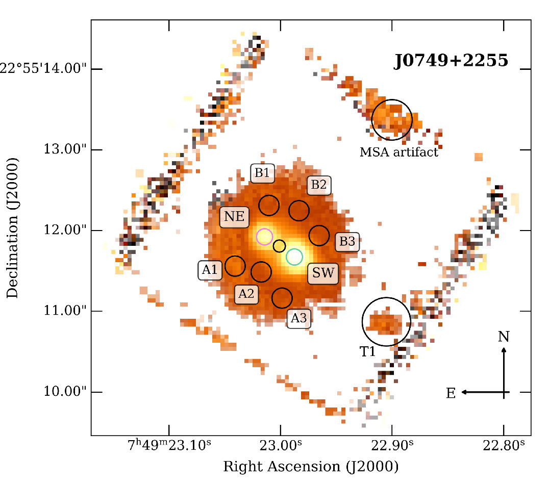
Figure 1: A map of the flux detected around the Hɑ and [NII] lines in the J0749+2255 system. The two quasars are found in the central region, denoted with “NE” and “SW.” [Adapted from Ishikawa et al. 2025]
Seeing Double?
Figure 2 shows the spectra for the SW and NE quasars, and the first thing that is impossible to ignore is just how similar they are. There are some small differences; for example, the NE quasar is slightly redder than the SW quasar, and some emission lines have different shapes and are a smidge offset from one another. But the general similarity brings up the possibility that what we’re looking at isn’t two separate quasars, but rather one object that’s being gravitationally lensed! The small differences in the spectra could be consistent with a lensing scenario, as they could be explained by time delays in the lensing or foreground contamination. A major problem with this idea, however, is that no observations of this system have provided evidence for a lens: we have not seen the massive foreground object that would actually be causing the gravitational lensing. While it’s possible that the lens is just incredibly faint, there’s no smoking gun for lensing happening here.
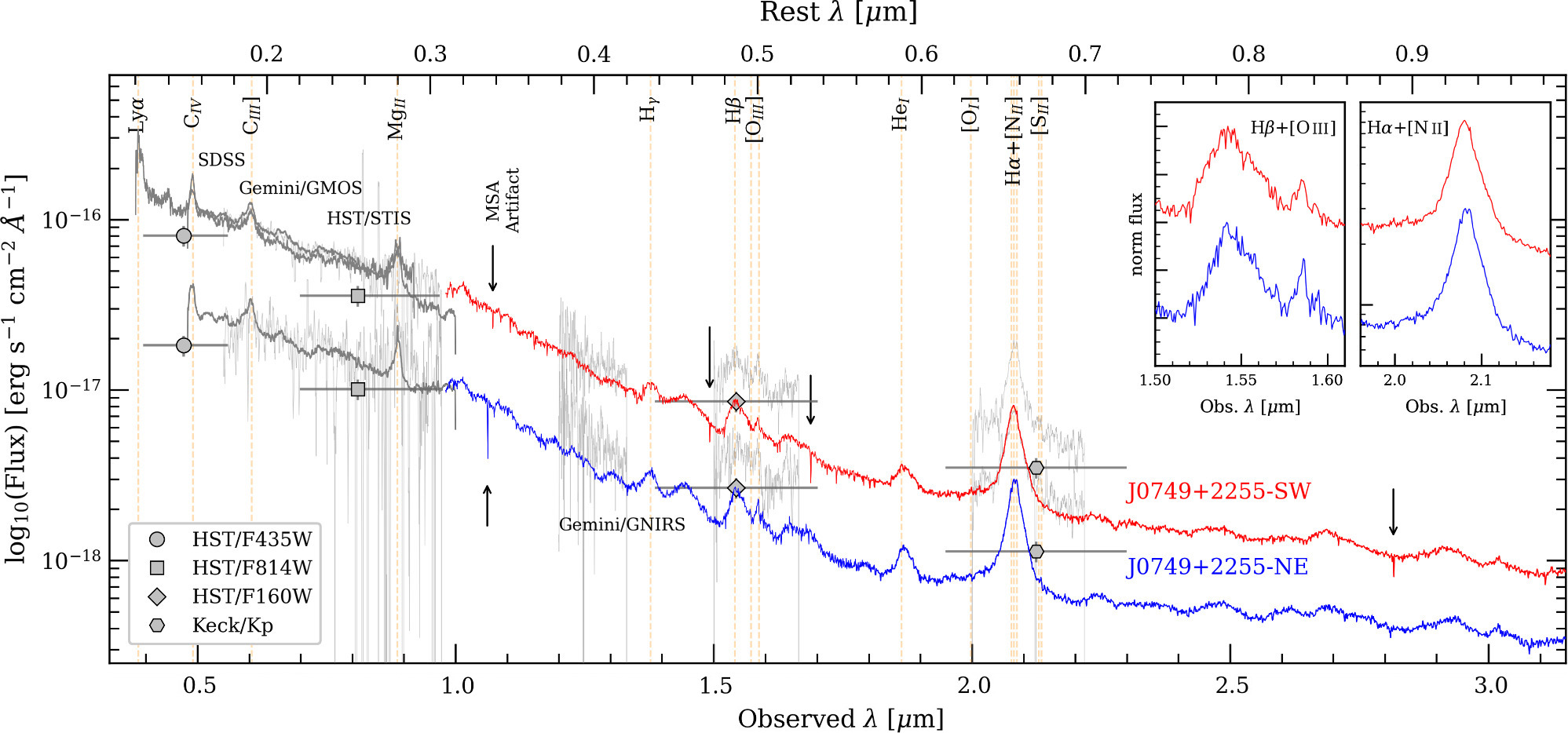
Figure 2: Spectral observations of the two quasars, vertically offset for clarity. The blue and red curves represent JWST observations, with the gray lines representing observations from previous works with other telescopes. The JWST results shown here demonstrate the remarkable similarity between the two quasars. [Adapted from Ishikawa et al. 2025]
Disk Gas Enters the Chat
The story becomes even more complicated when you look beyond the quasars, as JWST observations also detected diffuse emission from gas as shown in Figure 3. This gas is at the same redshift as the quasars, and can thus be associated with their host galaxy. And crucially, this gas doesn’t show any signs of lensing, such as the distinct arcs or symmetry you find in other lensed systems. This, coupled with the differences in the quasar spectra, suggests that this is not a lensed system, and that in fact we are looking at two different quasars.
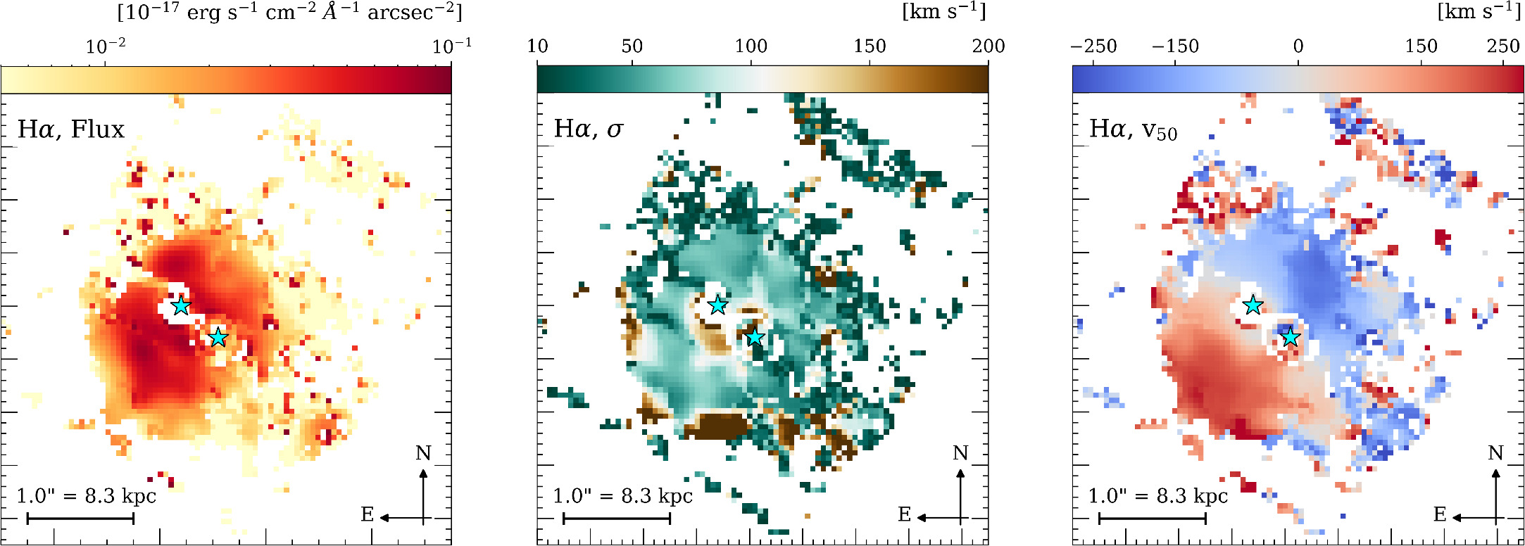
Figure 3: Maps of Hɑ emission with the quasar contributions removed. Left panel shows the flux, middle shows the velocity dispersion, and right the radial velocity. The radial velocity measurements provide strong evidence for a disk with gas rotation and relatively little disturbance, which is not usually the case for merger environments. [Ishikawa et al. 2025]
However, this story is complicated by the dynamics within the gas surrounding the quasars. As shown in the rightmost panel of Figure 3, the quasars are embedded in a gas disk that’s rotating, with one half of the gas being redshifted and the other half blue shifted. The quasars aren’t separated into these two regions, but are rather both found at the center of the disk. And the gas is showing none of the kinematic disturbance we would expect during a major merger, as the disk seems to be relatively stable. So maybe we’re not witnessing a merger in progress, but rather a disk galaxy that is playing host to two quasars! Based on simulations, one way this could happen is if a major merger takes place at an earlier time, and two black holes form from the resulting instabilities. This is another possible explanation for why the quasars are so similar.
Overall, this work points to the complicated nature of dual quasar systems. Is this one quasar being lensed or two different quasars? If they are distinct objects, are we witnessing a merger of galaxies, or did they both form in one galaxy? Future observations may be the key to answering these questions, but for now it remains a very interesting system.
Original astrobite edited by Hillary Andales.
About the author, Skylar Grayson:
Skylar Grayson is an astrophysics PhD candidate and NSF Graduate Research Fellow at Arizona State University. Her primary research focuses on active galactic nucleus feedback processes in cosmological simulations. She also works in astronomy education research, studying online learners in both undergraduate and free-choice environments. In her free time, Skylar keeps herself busy doing science communication on social media, playing drums and guitar, and crocheting!


bursts onto the Scene!")
 Nothing to See")