Supernova Archeology with Radioactive Eyes
Editor’s note: Astrobites is a graduate-student-run organization that digests astrophysical literature for undergraduate students. As part of the partnership between the AAS and astrobites, we occasionally repost astrobites content here at AAS Nova. We hope you enjoy this post from astrobites; the original can be viewed at astrobites.org!
Title: The distribution of radioactive 44Ti in Cassiopeia A
Authors: Brian Grefenstette et al.
First Author’s Institution: California Institute of Technology
Status: Published in ApJ
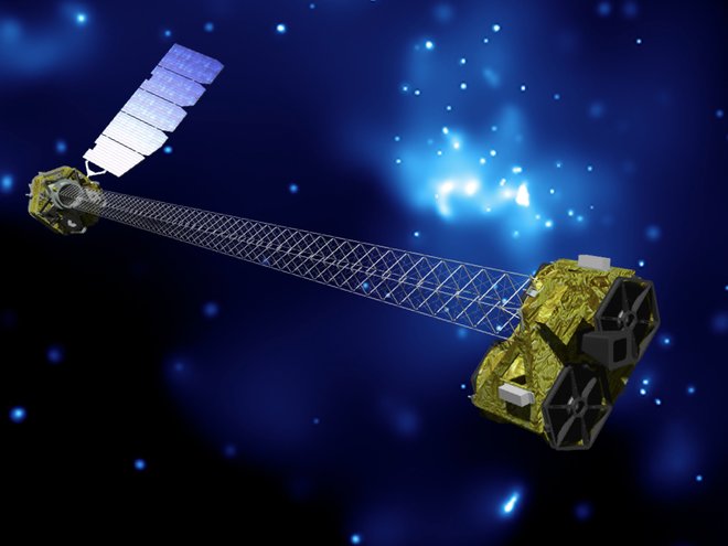
Artist’s concept of the NuSTAR X-ray satellite.
Massive stars die as core-collapse supernovae: the star can no longer produce the nuclear reactions that balance its strong gravity, and the star collapses onto its core. When this happens, large amounts of energy and neutrons are available to form elements heavier than iron. The distribution of elements produced in the deepest layers of the star as it goes supernova is key to understanding the mechanism by which the collapse of the star leads to an explosion. Radioactive decay powers the optical light emitted by the supernova around 50−100 days after the explosion. In fact, we can still see radioactive signatures in remnants that are hundreds of years old. In today’s paper, the authors use observations from the high energy X-ray satellite NuSTAR to study the distribution of 44Ti in the young supernova remnant Cassiopeia A (Cas A). The current distribution of radioactive elements and their decay products is linked to the local conditions in which they were synthesised when the explosion took place. Therefore, knowing where the 44Ti is now can shed light on the details of the supernova event that ended the life of Cas A’s progenitor star.
The Cas A Supernova Remnant
Cas A is known by radio astronomers as one of the brightest radio sources in the sky, although the bulk of its energy is emitted as thermal X-rays. These are produced as the ejecta from the star encounter the supernova remnant shock, and it heats them to X-ray emitting temperatures. Shocks are transition layers in which the thermodynamic properties of a plasma change rapidly; they arise whenever some material moves faster than the local speed of sound. Supernova remnants can show two kinds of shocks: the forward shock, which is the blast wave from the supernova explosion, and a reverse shock that forms as the forward shock bounces back when it encounters dense circumstellar material. We think Cas A’s explosion date is 1672, although there are no definite records of it being observed. It is one of the few historical supernova remnants found to be of type IIb from its light echoes (read this Astrobite for the details of supernova classification and this Astrobite to find out what makes light echoes such a mind-blowing astronomical technique).
Radioactive Elements and the Explosion
The production of radioactive elements is very sensitive to local conditions of density and temperature during explosive nucleosynthesis and can give us clues on the nature of the explosion mechanism. 44Ti has a half life of ~58 years, which means there is still a small amount of 44Ti in Cas A decaying. We can see these decays as high-energy lines within the frequency range of NuSTAR. In fact, the mass of 44Ti we measure today is directly proportional to its original mass, independent of what has happened to the ejecta in the 340 years since explosion. Another important radioactive product of explosive nucleosynthesis is 56Ni. Unlike 44Ti, 56Ni has a short half-life, ~6 days, which means we can only know its original abundance from the abundance of its stable decay product 56Fe.
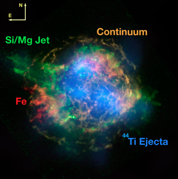
Figure 1: X-ray features of Cas A. The thin rim in the outermost layer is continuum synchrotron emission from the forward shock. Note that much of the X-ray emission forms a bright circle. This is because the ejecta are being heated by the reverse shock, which was generated when the supernova blast wave ran into the surrounding interstellar medium. [Robert Hurt, NASA/JPL-Caltech]
The authors find that almost all of the 44Ti is moving in the opposite direction of Cas A’s central compact object (CCO). The CCO is a neutron star that we think is the compact remnant of the supernova explosion. It is off-centre, so we believe that it received a ‘kick’ at the time of the explosion. Since the 44Ti is moving in the opposite direction, it can be part of the material that gave the neutron star its kick (from momentum conservation). They also find that there are regions where they see 44Ti and Fe, regions with 44Ti and no Fe, and regions with Fe and no 44Ti (recall that Fe is the decay product of 56Ni). Since the ratio of 56Ni to 44Ti is sensitive to the local conditions during the explosion, these observations suggest that the local conditions of the supernova shock during explosive nucleosynthesis were varied, and so there were large-scale asymmetries in densities of the innermost ejecta when the star went supernova.
Perhaps it is not so surprising that core-collapse supernovae are complicated events. In the case of Cas A, 4–6 solar masses of material collapsed on itself, with part of it forming a neutron star and part of it being expelled outward to interact with the medium around it. The asymmetries evident from element distributions result in a shell that is surprisingly spherical. There are clearly many details left to iron out as to how all of this happens. Works such as this one can offer us a (radioactive) glimpse into how it all fits together.
About the author, Maria Arias:
Today’s post was written by an Astrobites guest author: Maria Arias, a third year PhD student at the University of Amsterdam. She studies supernova remnants at low radio frequencies with the LOFAR telescope. She’s always happy to take a break from data reduction, though, and go for a yoga class, a run, or a beer.


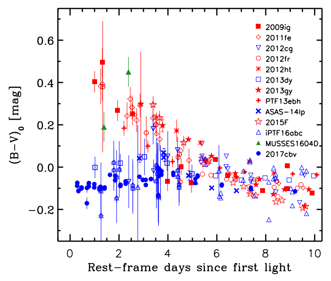
: Two Sub-Populations of Type Ia Supernovae?")