Astrobites RSS

illustration of the structure of the Milky Way

Editor’s Note: Astrobites is a graduate-student-run organization that digests astrophysical literature for undergraduate students. As part of the partnership between the AAS and astrobites, we occasionally repost astrobites content here at AAS Nova. We hope you enjoy this post from astrobites; the original can be viewed at astrobites.org.

Title: SPLUS J142445.34-254247.1: An r-process-enhanced, Actinide-Boost, Extremely Metal-Poor Star Observed with GHOST
Authors: Vinicius M. Placco et al.
First Author’s Institution: NSF’s National Optical-Infrared Astronomy Research Laboratory (NOIRLab)
Status: Published in ApJ

Have you ever looked at the periodic table and wondered where all the elements come from? Nearly all of the hydrogen, helium, and some of the lithium present in the universe formed in the first three minutes after the Big Bang. Beyond that, most of the elements (those that are heavier than helium are called metals by astronomers) were created in nuclear reactions that take place in the heart of stars. Up through iron, the formation processes happened systematically, where heavier elements were formed from the fusion of lighter elements. Beyond iron, about half of the elements are created by a slow and gradual process of capturing neutrons (called the s process, with s for slow).

Elements beyond iron are created in extreme events, such as stellar explosions (see Figure 1 for an overview). Such cataclysmic events cause neutrons to rapidly bombard atomic nuclei, forming heavier elements. This rapid capture of neutrons is called the r process (with r for rapid). There is a constant exchange of elements between the stars and the gas surrounding them. This eventually leads to the formation of more stars that are enriched in metals, setting up different generations of stars.

periodic table of the elements indicating the origins of each element

Figure 1: The astronomer’s periodic table indicates the elements’ astrophysical origin. [NASA’s Goddard Space Flight Center]

Studying the s and r processes can give us valuable insight into the nature and conditions prevalent in the universe when stars form. The s-process elements are believed to originate from low-mass stars as they evolve throughout their lifetime. The r-process elements come from dramatic events, such as supernovae or neutron star mergers. The mechanism through which a star’s r-process elements were created is determined mainly by modeling, as direct observational evidence of such events is rare.

If we obtain high-resolution spectroscopy of a star and map the abundances of all its elements, it would paint a picture of the events that led to its formation. In today’s article, the authors try to understand how stars were formed in the halo of the Milky Way by recreating the formation scenario based on the fingerprints in the high-resolution spectrum obtained from a Milky Way halo star called SPLUS J142445.34–254247.1, or SPLUS J1424−2542 for short.

Recreating the Formation Scenario

The star’s chemical abundances are determined from absorption features in its spectrum. If a particular element is present, it will absorb the starlight passing through the cold gas at a characteristic wavelength, and the extent of absorption can be used to determine how much of the element is present in the star. Looking at the elemental abundances of SPLUS J1424−2542, the star showed signs of being poor in iron (atomic number Z = 26) but being enhanced in elements with atomic numbers 26 < Z < 38 compared to the standard values measured from the Sun. This indicates the star formed from a gas cloud polluted by two distinct populations of stars in a multi-enriched process.

The abundances of the heavier elements indicate that the primary process involved in the formation is the r process. This is not uncommon for old stars in the galactic halo. The s-process elements are formed from the death of low-mass stars, which would not have occurred when such old stars were formed in the halo. Most elements in halo stars are created through the r process, even those typically formed by the s process. However, the authors found that certain elements, such as strontium, do not agree with the predicted values from either the r process or s process (Figure 2). Other elements, such as barium, are overproduced, indicating contributions from both s and r processes. The team also found an overabundance of thorium, which could indicate a possible contribution from a separate r-process event. Thus, this star is metal poor with enhanced heavy elements produced by r-process events.

observed elemental abundances compared to expected values from the r process and the s process

Figure 2: Observed abundances (red circles) with the expected values from the r process (blue line) and s process (yellow line). Most points lie on the blue line, indicating a more significant contribution from the r process. [Placco et al. 2023]

Modeling the formation scenarios predicts that the lighter elements (Z ≤ 30) were likely produced by a metal-free star with a mass in the 11.3–13.4-solar-mass range that exploded with low energies, a characteristic property of older Population III stars. The heavier elements (Z ≥ 38) were likely formed from the merger of two neutron stars with masses of 1.66 and 1.27 solar masses, indicating that at least two progenitor populations enriched the star.

Mysterious Circumstances Prevail

The authors derived the star’s kinematic properties (such as orbital dynamics, velocities, etc.), which are displayed in Figure 3. They found that the proposed formation scenario and the derived kinematics do not connect the star with any known structure in the Milky Way. This highlights that a distinct star formation mechanism may occur in the galactic halo. We must continue studying similar stars with high-resolution spectroscopy to help us understand the formation of old stars in the Milky Way halo.

comparison of the properties of the star studied in this article to those of stars in known Milky Way substructures

Figure 3: The yellow star indicates the star studied in this article. The upper panel shows it does not fall into the expected Milky Way streams. The bottom panel shows that it has distinct properties from other stars in a similar position on the upper panel. [Placco et al. 2023]

Original astrobite edited by Roel Lefever.

About the author, Archana Aravindan:

I am a PhD candidate at the University of California, Riverside, where I study black hole activity in small galaxies. When I am not looking through some incredible telescopes, you can usually find me reading, thinking about policy, or learning a cool language!

illustration of planets around an M-dwarf star

Editor’s Note: Astrobites is a graduate-student-run organization that digests astrophysical literature for undergraduate students. As part of the partnership between the AAS and astrobites, we occasionally repost astrobites content here at AAS Nova. We hope you enjoy this post from astrobites; the original can be viewed at astrobites.org.

Title: A Comparison of the Composition of Planets in Single-planet and Multiplanet Systems Orbiting M dwarfs
Authors: Romy Rodríguez Martínez et al.
First Author’s Institution: The Ohio State University
Status: Published in AJ

The most common type of star in the universe is the M dwarf, making up ~70% of all stars. Because M dwarfs are so common, and because we know exoplanets are common, it is only natural that we have found many exoplanets orbiting M-dwarf stars. In fact, Astrobites covered seminal articles on the occurrence rate of planets around M dwarfs and their compositions; read them here and here. But with all these planets, we can take our knowledge one step further and begin to ask deeper questions. For example, in M-dwarf planetary systems, how do single-planet systems (only child) and multi-planet systems (siblings) compare?

A new study seeks to answer this question, focusing on three key parameters: planet bulk density, planet core mass fraction, and host-star metallicity. In particular, the authors wish to investigate whether siblings and only-child systems are two outcomes of the same formation process, or if they truly form differently. In other words, are they from the same population, or are they two distinct populations of planets?

Bulk Density

First, bulk density, or the average density of the planet as a whole. We know that Earth is made up of many different materials (rocks, water, gases, etc.) and each one of these has its own density. But for exoplanets, we cannot explore the details of different materials and so instead we measure bulk density by simply taking the total mass of the planet and dividing by the total volume (assuming the planet is a sphere). The authors compute bulk density for a sample of planets around M dwarfs, computing this quantity for both the single-planet systems and all the planets in multi-planet systems.

Next they apply a statistical test (the Kolmogorov–Smirnov test) to determine if the two sets of planets are truly distinct populations or are consistent with one population (see Figure 1 top panel). The result overwhelmingly shows that these are two different populations. However, the authors caution that this result may be biased. Many of the single-planet systems in the sample are giant planets, which are naturally lower density than smaller planets are because they have higher gas fractions. Removing the gas giants from the sample and re-running the test, the authors find that actually the siblings and only-child planets are consistent with coming from the same population (see Figure 1 bottom panel).

plots of cumulative distribution function vs planet density

Figure 1: Top: The results of the statistical test when including all planets to determine if the two populations are distinct. The gap between the single and multis suggests they are indeed two populations. Bottom: The same as the top panel but for the sample that excludes giant planets. Here the finding of two populations is less statistically significant. [Adapted from Martínez et al. 2023]

Core Mass

Next, planet core mass. The mass of a planet is generally meant to include everything that makes up the planet. However, the core mass is just that, the mass of the core of the planet alone. Core masses are valuable pieces of information because it is thought that the size of the core, which is the first to form, can determine how big the planet eventually grows to be. Bigger cores are better at gravitationally attracting material, including gas, to grow the planet. While we cannot directly measure the core mass of a planet, we can use models that are tuned to Earth’s parameters to estimate planet core mass based on a few things we can measure, like mass and radius. Now taking only the planets that are likely to be rocky and again splitting by single versus multi-planet systems, the authors find that planets in single-planet systems have, on average, larger core masses than those in multi-planet systems. They further test if core mass correlates with orbital period but find no correlation.

Metallicity

Lastly, the authors explore the host star, particularly its metallicity, or the percentage of the star’s composition that is made up of “metals” (astronomers define “metal” as anything heavier than helium!). Host star metallicity is thought to correlate with the kinds of planets and number of planets in the system, the thinking being that since planets form out of the same disk of material as the host star, if there are more heavy materials in that disk (which would appear as higher metallicity in the host star) then there is more opportunity to make more and bigger planets. The authors here find that host stars of single planets are more metal rich than those hosts of multi-planet systems. This is counterintuitive, but the authors hypothesize this could be because more metal-rich stars might produce more and bigger planets, which may gravitationally interact in the early days of the system and fling out all but one planet. On the other hand, metal-poor stars cannot build big planets and instead build small planets that are dynamically “quiet.”

In all, the authors find that single- and multi-planet M-dwarf systems are likely two distinct populations. This could have large implications for how we understand the formation and evolution of planetary systems.

Original astrobite edited by Mark Popinchalk.

About the author, Jack Lubin:

Jack received his PhD in astrophysics from UC Irvine and is now a postdoc at UCLA. His research focuses on exoplanet detection and characterization, primarily using the radial-velocity method. He enjoys communicating science and encourages everyone to be an observer of the world around them.

a photograph of the Sun and an illustration of a pulsar

Editor’s Note: Astrobites is a graduate-student-run organization that digests astrophysical literature for undergraduate students. As part of the partnership between the AAS and astrobites, we occasionally repost astrobites content here at AAS Nova. We hope you enjoy this post from astrobites; the original can be viewed at astrobites.org.

Title: Probing the Solar Interior with Lensed Gravitational Waves from Known Pulsars
Authors: Ryuichi Takahashi
First Author’s Institution: Hirosaki University
Status: Published in ApJ

Forget X-ray vision — how about gravitational wave vision? In today’s article, a team of researchers examine the possibility of using gravitational waves from distant pulsars to learn about our own Sun. Much like the terrestrial seismologists and geologists who peer into Earth by listening carefully to the ways waves are distorted as they travel through its many layers, these imagined future gravitational heliophysicists would use the subtle distortions of gravitational waves that have passed through the Sun to learn about its inner contents.

Multi-messenger Seismology?

The idea of using the interaction between waves and normal matter to peer under the surface of otherwise opaque objects has a longstanding history in physics. Think for example of the idea of seismic tomography, one of the main tools used by seismologists and geologists to understand the makeup of Earth’s interior. As powerful shock waves move through Earth’s interior after seismic events like earthquakes, they come into contact with regions of material that may differ in their composition, density, temperature, and so on. Depending on the wave frequencies and the properties of the materials with which the waves come into contact, these waves will reflect, refract, diffract, or be otherwise altered from their initial waveform. Measuring the properties of these waves when they make contact with the surface again at different points around the world can thus tell us a great deal about what they may have encountered on their journey through the depths.

Similarly, when electromagnetic waves (light) encounter solid objects, they can undergo a number of interactions: certain wavelengths will be scattered or absorbed, and others may pass directly through an object. This is, roughly speaking, how X-ray imaging works: certain high-frequency electromagnetic rays can easily pass directly through your soft skin, but they will be reflected upon encountering denser material like bones, allowing us to reconstruct images of the interior of our own bodies without the need for invasive surgeries (thanks, science!).

Today’s article examines the feasibility of doing similar reconstructions but with waves of a different kind: gravitational waves. Gravitational waves, which have been discussed at length in previous Astrobites, are a hot topic right now within the astrophysics community given that the technology to directly detect their subtle presence has only come to maturity within the past decade or so. This is because gravitational waves, which are produced by the asymmetric motion of massive objects like black holes in binary orbits, produce extremely subtle effects here on Earth due in part to the weakness of the gravitational force and in part to the large distances the waves have typically traversed to reach us. Now that we are measuring these faint signals with regularity in ground-based gravitational wave detectors like LIGO, VIRGO, and KAGRA, interest has been growing in finding more and more exotic ways to use this brand new window into the universe to uncover its many secrets.

To understand the particularly out-there idea behind today’s article, we need to introduce at least one further concept: gravitational lensing. Gravitational lensing occurs when particles (or waves) travel close to a massive source and as a result have their trajectories altered. When a massive source (like a galaxy cluster) sits more or less directly between Earth and some distant object (like an individual galaxy), this deflection can act like a lens, focusing the light from the background galaxy towards Earth to make the galaxy appear bigger, brighter, or even more emoji-like. Additionally, as waves of any kind travel past such a lens, they will appear to take longer to reach the other side than they would have if there were no massive source. This effect is known as gravitational time delay, and it can sometimes manifest in ways not too dissimilar from the way in which light appears to “slow down” when passing through dense mediums like water. Gravitational lensing can cause all sorts of waves including gravitational waves to undergo many distorting effects similar to light traveling through media of varying densities or seismic waves traveling through Earth’s interior.

Taking all of these effects into account, we can begin to see why the idea of using gravitational waves to probe the interior of the Sun isn’t so far-fetched. While electromagnetic waves cannot typically pass into and out of the Sun due to their interactions with dense solar material, gravitational waves from a source behind the Sun would pass through easily, only experiencing distortion due to the aforementioned lensing effects caused by the varying density of the Sun along the line of sight between detectors on Earth and the source of the gravitational waves. While this idea has been explored before, today’s authors attempted a comprehensive analysis of what these distortions might look like for a set of real sources and examined how feasible it would actually be to detect them in present or future gravitational wave observatories. So can it be done? As it turns out, with some upgraded detectors, a dash of new millisecond (very fast-spinning) pulsar discoveries, and a bit of luck — it can!

Looking for Magic Millimeter Mountains

diagram showing the alignment of Earth, the Sun, and a distance source of gravitational waves that passes directly behind the Sun

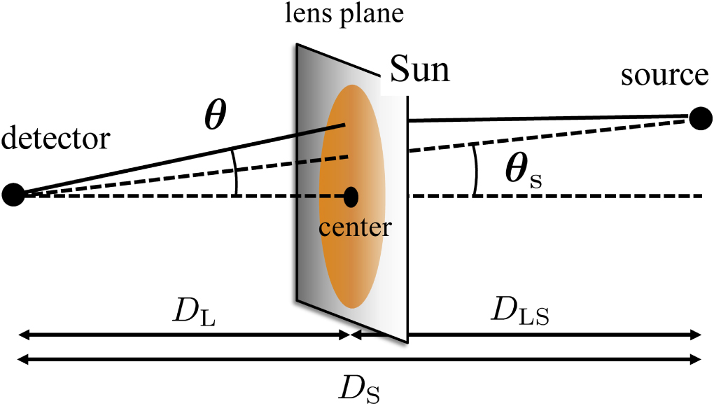
Figure 1: Depiction of the arrangement of an Earth-based gravitational wave detector and an object that emits continuous gravitational waves that is of interest to the authors of today’s article. When gravitational waves from the source have to pass directly through the Sun to reach Earth, they can be deflected from their original path and distorted in ways similar to how light is distorted when passing through a traditional lens. [Takahashi et al. 2023]

Unlike with light waves or even some seismic waves, humans do not have the capacity to generate gravitational waves of sufficient power to be measured and manipulated for the purposes of doing experiments. Instead, if we want to use these new waves to our benefit, we have to get clever with what nature has provided for us. Firstly, what we will need is a source of continuous gravitational waves. Unlike most of what LIGO sees right now, which are the signature “chirps” of compact objects undergoing their last seconds of merging, the continuous waves (meaning gravitational wave signals that are continuously emitted from a source and detectable for some appreciable amount of time) that are expected to be seen by ground-based detectors are most likely to come from tiny (sub-millimeter scale) deformations (sometimes called “mountains”) on the surface of rapidly rotating pulsars. Once gravitational wave detectors increase in sensitivity enough to finally detect these waves, researchers will want to find sources that occasionally pass behind the Sun from our perspective here on Earth (Figure 1). Over the course of several hours as Earth moves along its orbit, detectors on Earth may be able to observe how this continuous signal changes as it appears to pass behind different parts of the Sun, like watching a straw appear to bend when lowered into a glass of water.

The authors of today’s article employ mathematical formulas (that are not too dissimilar from what one would see in an introductory optics course!) to calculate the amount of deflection, convergence, and time delay experienced by gravitational waves passing behind the face of the Sun at various angles relative to its center. Further wave-optics calculations are employed to find the corresponding amplification factors and phase offsets that waves of different frequencies would experience at these various angles. Their results are clearly shown in Figure 2: as each candidate pulsar (labeled by the different colored lines) appears to pass behind the face of the Sun, its corresponding gravitational wave signal will be amplified and offset in phase in complicated ways determined in part by the frequency of each gravitational wave and how closely the signal gets to passing directly behind the center of the Sun. By understanding how strong these effects are for continuous waves with different frequencies and amplitudes, the authors can begin to assess what it will take to detect them.

modeled amplification and phase offset of a gravitational wave signal passing behind the Sun from our perspective

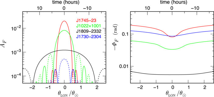
Figure 2: Models for the amplification (left) and phase offset (right) of a potential continuous wave signal as their line of sight appears to pass behind the Sun from four pulsars that are known to be eclipsed in this way once each year. [Takahashi et al. 2023]

As it turns out, the ideal continuous-wave-emitting pulsars are those with high rotational frequencies (>10 Hz) that pass as close behind the Sun’s center as possible. When applying this cutoff to catalogs of known pulsars, only four currently fit the bill. While this doesn’t sound ideal, the authors go on to acknowledge that there are expected to be thousands more fast-spinning millisecond pulsars within our own galaxy that we have yet to discover, many of which could also turn out to pass behind the Sun on occasion.

diagram of the locations of annuli used to estimate the solar density

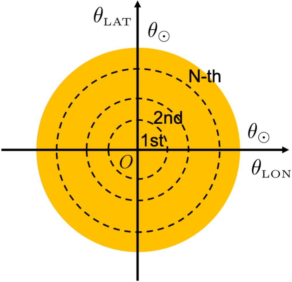
Figure 3: Estimates of the solar density profile will have to be made at different chosen slices called “annuli” (depicted here as the numbered concentric circles). Choices for how to pick these annuli affect how accurately their densities can be recovered for a given continuous wave pass. [Takahashi et al. 2023]

With all this background knowledge in hand, the primary question left to tackle is this: can these slight deformations in continuous waves actually be detected with enough confidence to infer the density of different layers of the Sun? As to whether the lensing signal could be detectable at all, the authors of today’s article find that such a detection could be made with a high degree of confidence using known pulsars with about one year’s worth of observation time given a signal-to-noise ratio of around 100 or greater. The signal-to-noise ratio can depend on many factors including the loudness of a given source, the sensitivity of the detector, and the timespan of data collection, but to put this number in perspective, current signal-to-noise ratio upper limits for continuous wave detections from LIGO searches are estimated to be around 10.

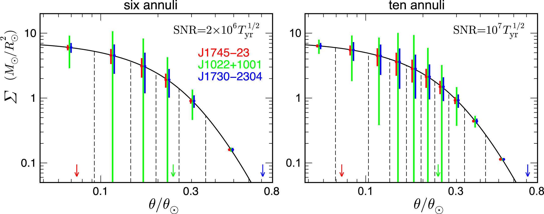
Unfortunately, accurately measuring the solar density at several different solar depths is even trickier, as the accuracy of each measurement depends on a variety of factors including how many total layers of the Sun one attempts to measure and how one sets the distance between each layer (Figure 3). For one year of continuous wave observation of the three best pulsar candidates, the signal-to-noise ratio needed to accurately measure the solar density at two different layers is found to be ~104, which is an order of magnitude higher than is even expected from the next-generation gravitational wave detectors Cosmic Explorer and the Einstein Telescope. To measure densities across 6 or 10 different layers of the Sun’s interior, the signal-to-noise ratio requirements grow to ~106 and ~107, respectively (Figure 4), well beyond the capabilities of planned detectors unless more rapidly spinning pulsars passing behind the Sun can be found and loudly heard in these future detectors.

uncertainty in solar density measurements at various solar depths using the expected lensing signatures of three known pulsars as they pass behind the Sun

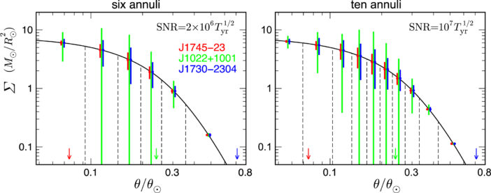
Figure 4: This plot depicts the uncertainty in solar density measurements at various solar depths using the expected lensing signatures of three known pulsars as they pass behind the Sun. The solid black line depicts the expected solar density as a function of solar radius (measured here as the angular position on the face of the Sun relative to its center). In the case where one attempts to measure six distinct densities with a very high signal-to-noise ratio of 106 over one year of observation (left plot), uncertainties can become fairly low close to or far away from the Sun’s center. To achieve similar uncertainties across 10 annuli, a comparative signal-to-noise ratio of 107 is necessary. [Takahashi et al. 2023]

Prospects for Gravitational Wave Vision

In recent years, combining gravitational waves with gravitational lensing has been proposed as a way to learn all sorts of new things about our universe, from constraints on the Hubble constant to independent measurements of the masses of distant stars. While it may take many more years for this sort of analysis to mature to a point where it can give us useful information about the Sun’s density profile, the fact that it may be possible at all is remarkable. For many decades the detection of gravitational waves was thought to be impossible. Now, not only are we detecting them with regularity, but we are finding all sorts of new ways to learn about our universe with each passing day — and that’s something to be excited about, even if you won’t be seeing gravitational wave vision goggles in stores anytime soon!

Original astrobite edited by Jessie Thwaites.

About the author, Lucas Brown:

I’m a current master’s student at Tufts University interested in cosmology, relativity, and gravitational physics. I am currently doing research on the stochastic gravitational wave background and pulsar timing arrays. Outside of physics I love playing piano, climbing, and spending time with my dog.

dusty star forming region

Editor’s Note: Astrobites is a graduate-student-run organization that digests astrophysical literature for undergraduate students. As part of the partnership between the AAS and astrobites, we occasionally repost astrobites content here at AAS Nova. We hope you enjoy this post from astrobites; the original can be viewed at astrobites.org.

Title: Spatially-Resolved Temperature and Density Structures of Nearby HII Regions
Authors: Yifei Jin et al.
First Author’s Institution: Australian National University
Status: Published in ApJ

Despite playing a fundamental role in shaping the emission-line spectra of HII regions, the assumptions about electron temperature and density that are used in most photoionization codes are oversimplified and quite far from reality. In today’s article, the authors analyzed the detailed electron temperature and density structures of four HII regions to show — spoiler alert! — that the prevailing assumptions are not physically realistic.

For Real

Photoionization, a key process in astrophysics, is the physical mechanism that converts electrically neutral atoms (or molecules) into ions through interactions with energetic photons. This phenomenon plays a crucial role in determining the characteristics of HII regions, where intense ultraviolet photons from massive stars lead to the ionization of the surrounding hydrogen gas.

Much of our knowledge about objects in the universe comes from spectroscopy (here is Astrobites’s Guide to Spectroscopy and Spectral Lines). The spectra of HII regions are dominated by emission lines that trace the characteristics of the emitting gas. Among the physical quantities influencing the emission-line spectra of HII regions are the electron temperature and density. These parameters serve as crucial diagnostics for determining the metallicities of the interstellar medium.

Reality Check

Diagram illustrating an idealized or simplified spherical HII region

Figure 1: Diagram illustrating an idealized or simplified spherical HII region. [AAS Nova/Kerry Hensley]

To interpret the spectra of HII regions and understand the complexities of such ionized environments, astronomers rely on photoionization codes. These codes model the interactions between the ionizing radiation emitted by the ionizing source(s) and the surrounding gas, and they provide insight into three key factors:

  • the nature of the central star
  • the physical conditions of the ionized nebula
  • the chemical abundances that characterize the nebula

Photoionization codes tend to underestimate the complexity of the internal nebular structures of HII regions by assuming an isothermal condition (constant temperature) or a uniform electron density distribution across the extent of these regions. Additionally, in most models, the nebular geometry is assumed to be spherically symmetric, a simplification that often does not align with the real objects — as is evident if you compare the HII-region diagram in Figure 1 with the images from observations of the four HII regions studied in the article in Figure 2!

What’s Real vs. The Models

The authors of today’s article utilized integral field unit data from the Wide-Field Spectrograph (WiFeS) on the Australian National University 2.3-meter telescope to analyze the detailed temperature and density structures of four HII regions in the Magellanic Clouds (Figure 2). Integral field unit instruments enable simultaneous imaging and spectroscopy observations, generating a spatially resolved data product called a data cube that contains spectral information at each spatial pixel (spaxel). This article represents the first investigation into the nebular internal structures with a sample of extragalactic HII regions using integral field unit data with a high spatial resolution.

images of four HII regions

Figure 2: Integrated-flux (in erg s-1 cm-2) images of the four HII regions with relative positions (in arcseconds), showcasing the different nebular morphologies. [Adapted from Jin et al. 2023]

The authors used the temperature-sensitive [O III] line ratio to derive electron temperatures from the data and the density-sensitive [O II] and [S II] line ratios for the electron densities. The MAPPINGS V photoionization code was employed to create models, incorporating stellar atmosphere libraries as input for the ionizing sources’ spectra and using spherical nebular geometry assumptions for the shapes of the HII regions. MAPPINGS V generated a set of HII-region models with line fluxes for all the emission lines within the set threshold (specified in the source file).

Figure 3 compares the radial profiles of the temperature- and density-sensitive line ratios between the observed and modeled values derived from the best-fit models (those with minimal χ2 values) for all four HII regions. The models predict that the density-sensitive [O II] and [S II] line ratios increase (top row) and remain flat (bottom row), respectively, with the distance from the center of the nebula. On the other hand, the observational data show a decreasing trend for [O II] line ratios, while [S II] ratios increase. Meanwhile, the observed radial profiles of the temperature-sensitive [O III] line ratios are flat (middle row) for all four regions, but the models predict decreasing profiles. These discrepancies suggest that none of the simple HII-region models is able to reproduce the observed electron temperature and density structures.

plots of radial distribution of line ratios in H II regions

Figure 3: The [O II], [O III], and [S II] line ratios as functions of normalized radius of the nebula with 0.0 being the center of the nebula. The yellow points represent the values from the observational data and the red dashed lines show the modeled radial distribution. [Adapted from Jin et al. 2023]

Let’s Be Real

Real HII regions exhibit notable radial variations in electron temperatures and densities, challenging the isothermal and/or constant density assumptions in photoionization codes. Codes like MAPPINGS V require assumptions about the shape of HII regions as input. Today’s authors have demonstrated in their article the pressing need to model realistic HII regions for accurate nebula modeling, emphasizing the importance of considering the arbitrary geometries inherent in these regions. As our understanding advances, the demand for a more realistic modeling approach grows. Ongoing developments in three-dimensional photoionization codes with Monte Carlo radiative transfer techniques (for more reading about the basic principle of this technique, this page is a good start) hold the promise of a new era in astrophysical simulations, providing a more physically realistic portrayal of these fascinating objects!

Original astrobite edited by Roel Lefever.

About the author, Janette Suherli:

Janette is a PhD student at University of Manitoba in Winnipeg (Winterpeg!), Canada. Her research focuses on the utilization of integral field spectroscopy for the studies of supernova remnants and their compact objects in the optical. She grew up in Indonesia where it is summer all year round! Before pursuing her PhD in astrophysics, Janette worked as a data analyst for a big Indonesian tech company, combating credit card fraud.

image of interacting galaxies

Editor’s Note: Astrobites is a graduate-student-run organization that digests astrophysical literature for undergraduate students. As part of the partnership between the AAS and astrobites, we occasionally repost astrobites content here at AAS Nova. We hope you enjoy this post from astrobites; the original can be viewed at astrobites.org.

Title: Revisiting Galaxy Evolution in Morphology in the COSMOS field (COSMOS-ReGEM): I. Merging Galaxies
Authors: Jian Ren et al.
First Author’s Institution: Chinese Academy of Sciences
Status: Published in ApJ

Galaxies are a bit like LEGO. At least, if you simplify down one of the fundamental theories of Lambda-CDM cosmology, our current best model of the universe, what you could say is that all structures in the universe today formed from the merging of smaller structures, much like building up a LEGO masterpiece. So, to build a massive galaxy like our own Milky Way, you need to merge lots of smaller galaxies together first (e.g., see this bite). One day, our galaxy will collide with our nearest neighbour, the Andromeda Galaxy, to form an even more massive galaxy. If you wind back the clock of our universe, what this simple, fundamental idea predicts is that galaxy collisions were more frequent back in the early universe. However, this has been a difficult prediction to prove as it requires observations much deeper into the universe.

Whilst it might seem easy to identify these colossal collisions with nearby galaxies, this gets very difficult for more distant galaxies, i.e., galaxies in the early universe (since distant = higher redshift = longer lookback time). At these distances, we need better instruments and bigger telescopes to resolve enough detail and collect enough light to really identify these more distant and therefore fainter mergers. The authors of today’s article have used observations of the Cosmic Evolution Survey (COSMOS) field — an area of the sky that has been extensively observed by multiple cutting-edge telescopes — to identify merging galaxies and investigate their properties.

How to Spot a Merger

There are a variety of different methods to identify merging galaxies. If you have sufficient spatial resolution, meaning you can see the extent of a galaxy rather than just a point source, you often see the evidence just by eye. In the featured image above, you can see a beautiful example of a local merger. These are called the Mice Galaxies, or NGC 4676. This merger is close enough for us to see it in action — the two galactic nuclei are clearly distinguishable, and we can even see a bridge connecting the two, as well as bright tidal tails of stars and gas streaming away from the collision. The authors of today’s article identified similar features in the COSMOS field. Some examples of these features are shown in Figure 1. In total, they identified 3,594 galaxies out of 33,605 galaxies as mergers by visually inspecting the images and searching for these clues.

images of merging galaxy pairs

Figure 1: Examples of some merging galaxies visually identified in this article. Each square is a different pair of merging galaxies. Each pair is at a different redshift, z, and stellar mass. [Ren et al. 2023]

Alternatively, you can also search for galaxies that are close together, since the expectation is that gravity will already be pulling these galaxies toward an imminent collision. This is useful if you can’t resolve much detail about the galaxies and can only see them as point sources. However, it is not enough to just find two points of light that look close together on an image; if you look up at a patch of the night sky, you might see two galaxies that appear close together, but in reality, one galaxy could be a million times farther away from us than the other. To check for this pesky problem, you need to know the redshift of the galaxy (again, remember that redshift is often used as a measure of distance from us, the observers). By checking the distances between sources in both the two-dimensional plane of the sky and according to their redshift, the authors identified 1,737 galaxy pairs.

Sometimes, however, even this method is too difficult. Redshifts can be hard to obtain (e.g., see this bite) and sometimes distances are just too great to even resolve galaxy pairs. For this reason, today’s authors used their impressively huge sample of mergers, pairs, and non-interacting galaxies to investigate some alternative methods that could be useful for a higher-redshift sample. They find that two parameters in particular, M20 and A0, are especially good at identifying mergers. M20 is a measure of how the brightness is spread across a galaxy, and A0 measures the asymmetry of the outskirts of a galaxy. The images of merging galaxies typically have much higher M20 and A0 values than the images of non-merging galaxies. This makes some sense — merging galaxies should show much less structure and symmetry since these collisions are violent and chaotic.

Mergers Across Cosmic Time

plot of merger fraction over cosmic time

Figure 2: How the merger fraction, which is calculated according to the visually identified mergers (blue points) and the number of pairs (black points), varies as a function of redshift, z. Estimates from other works are also shown. Click to enlarge. [Adapted from Ren et al. 2023]

The merging galaxies identified in this work span a redshift range of z = 0.2–1 — in terms of time, that’s from 2 billion to 8 billion years ago. Counting up all of the galaxies detected in the article’s observations, and labelling them as merging or not merging via the above methods, we can see in Figure 2 that the merger fraction (number of mergers out of the total galaxy sample) increases as a function of redshift. As predicted, there are indeed more mergers earlier in the universe. From this evolution, it is estimated that a massive galaxy in the redshift z < 1 universe will experience, on average, one major merger every 10 billion years.

Future efforts by the next generation of cutting-edge telescopes, as already begun by JWST, will help to extend this investigation to higher and higher redshifts. Seeing back earlier in time will paint a picture of galaxy mergers at the beginning of the universe, where the cosmic game of LEGO was likely even more intense and chaotic.

Original astrobite edited by Storm Colloms.

About the author, Lucie Rowland:

I’m a first-year PhD student at Leiden Observatory in the Netherlands, studying massive, star forming galaxies in the early universe with ALMA and JWST. It’s a really exciting time to be interested in astronomy, so I hope to make groundbreaking new research more accessible!

illustration of a planetary system

Editor’s Note: Astrobites is a graduate-student-run organization that digests astrophysical literature for undergraduate students. As part of the partnership between the AAS and astrobites, we occasionally repost astrobites content here at AAS Nova. We hope you enjoy this post from astrobites; the original can be viewed at astrobites.org.

Title: Can Cold Jupiters Sculpt the Edge-of-the-multis?
Authors: Nicole Sobski and Sarah Millholland
Authors’ Institutions: Wellesley College and Massachusetts Institute of Technology
Status: Published in ApJ

The Kepler mission revealed thousands of transiting exoplanets. Through this unique data set, we have come to understand much more about exoplanet demographics and the occurrence rates of different kinds of planets. In particular, we now understand that the most common type of planetary system is what we refer to as a “compact multi-planetary system.” That is to say, a system of multiple small planets (less than 4 Earth radii each) where each planet orbits in similar, short timespans (usually less than about 50 days). Studies of the full Kepler data set show that these “compact multis” are ubiquitous across the galaxy. Furthermore, these systems are shown to have a high rate of intra-system uniformity, sometimes called “peas-in-a-pod” architecture. Planets within a compact multi often have similar radii and similar spacing in their orbital periods.

But in a system of multiple transiting exoplanets of such uniformity, what causes the system to “end”? That is, what causes the pod to be filled up with peas? A new study looks into one possible force that may “sculpt” the edge of a compact multi-planet system: cold Jupiters. A cold Jupiter is a planet that has the mass of our own solar system’s Jupiter and is widely separated from its host star. The authors explore if and how the existence of a cold Jupiter at wide separation from an inner compact multi arrangement might determine how the pod gets filled with peas.

To test this, the authors needed a data set of known compact multis. They turned to the Kepler data set and selected the systems with at least four transiting planets. This left them with 279 planets in 64 systems. Next, they compiled the previously measured masses of these planets; only 60 of 279 had masses, so for the remainder they used a well-described mass–radius relationship to estimate planet masses. Planet mass is a crucial input for this study as mass is the primary parameter needed for dynamical studies, which inherently rely on gravitational forces.

To determine if and how a cold Jupiter could sculpt the edge of the inner compact system, the authors devised a dynamical study. Dynamical studies test how planets interact with each other through their gravitational influence on one another; often a researcher will test to see if a certain configuration of planets is stable or if it is unstable. In an unstable system, some or all of the planets get gravitationally kicked out of the system. Using a simulation software called the Stability of Planetary Orbital Configurations Klassifier (SPOCK), which takes in a list of planet masses and a few basic orbital parameters, the authors were able to compute the stability of the system over a specified time span. The authors added a simulated cold Jupiter (with parameters drawn from random distributions) to a planetary system with real planet masses and orbits and then determined the system’s stability over 1 billion years. For each of the 64 systems in the sample, they performed this test 10,000 times, noting the probability that the system was stable or not over that time span.

Each test resulted in one of three outcomes: unstable, fully stable, or metastable. Within the context of this study, metastable meant that the system was stable in about half of the simulations. Unstable simulations mean that the system will be ripped apart by gravitational interactions. The injected cold Jupiters that result in unstable configurations are not considered plausible edge-sculptors, then, because we do see planets in these systems; if the presence of a cold Jupiter made the system unstable, we wouldn’t see planets in the system. Next, the stable simulations represent injected cold Jupiters that had no effect on the inner system. These cold Jupiters exist at too wide a separation from the inner system for gravity to play a role in sculpting the edge of the pea pod. Therefore, these planets were also not considered plausible edge-sculptors. The metastable simulations, in which the odds of the system falling apart were between 30% and 70% (above 70% was considered fully stable), are the most interesting. These simulations correspond to systems in which the injected cold Jupiter had a real effect on the inner compact system and could potentially sculpt the edge of the inner compact system, as shown in Figure 1.

Plot of probability of stability as a function of perturber orbital distance and perturber mass

Figure 1: An example of the results of the main dynamical experiment for one multi-planet system. Each point is one of the 10,000 simulations where a cold Jupiter with randomized orbital parameters (y axis) and mass (x axis) is injected into the dynamical simulation along with the real planets. The dots are color coded by the probability of a stable configuration after 1 billion years: purple is unlikely to be stable, yellow is very likely stable. The metastable region is defined by the shading and red line. Because this particular system has a very small metastable region, it is highly unlikely that any cold Jupiter, if it exists, would play the role of the “edge sculptor.” [Adapted from Sobski & Millholland 2023]

However, looking at the mass and orbital parameters of the injected cold Jupiters that resulted in metastable simulations revealed a problem for the authors’ hypothesis: If these planets really existed in the Kepler systems tested, then observers should have been able to detect them in real data sets. These planets are large enough in radius that even accounting for transit probabilities, they likely would have been detected at appropriate rates in the Kepler data set. Similarly, they are massive enough and close enough to the inner system that radial-velocity surveys should easily detect them, but real radial-velocity data sets do not. (Radial-velocity surveys rely on measuring the Doppler shift of light due to a planet tugging on its host star.)

Therefore, the authors conclude that cold Jupiters likely do not help sculpt the edge of compact multi-planet systems. If they could, we would have found them in real data; since we don’t find them in real data, they must not exist in the compact multis studied here. Even though this experiment led to the rejection of the original hypothesis, it is nevertheless a fascinating result that tells us a bit more about the way exoplanet systems may form and evolve.

Original astrobite edited by Lindsay DeMarchi.

About the author, Jack Lubin:

Jack received his PhD in astrophysics from UC Irvine and is now a postdoc at UCLA. His research focuses on exoplanet detection and characterization, primarily using the radial-velocity method. He enjoys communicating science and encourages everyone to be an observer of the world around them.

dusty molecular clouds in the Carina Nebula

Editor’s Note: Astrobites is a graduate-student-run organization that digests astrophysical literature for undergraduate students. As part of the partnership between the AAS and astrobites, we occasionally repost astrobites content here at AAS Nova. We hope you enjoy this post from astrobites; the original can be viewed at astrobites.org.

Title: The Global Structure of Molecular Clouds: I. Trends with Mass and Star Formation Rate
Authors: Nia Imara and John C. Forbes
First Author’s Institution: University of California, Santa Cruz
Status: Published in ApJ

Molecular clouds are stellar nurseries, the birthplace of stars in our universe. These clouds are made up of cold molecular hydrogen, H2, which can clump together and collapse to form stars. Despite being such a vital part of the universe, the physics behind molecular clouds still needs to be better understood. Observations of molecular clouds provide limited information about their three-dimensional structure, making it challenging to study what exactly it is about these clouds that enable them to form stars.

Creating models that resemble molecular clouds is an excellent way to understand them in great detail. Comparing the models to actual observations enables us to tweak the model so that it matches all the observational properties of the object, thus letting us use the properties of the model to study the properties of the actual object.

So, how does one go about building a model of a molecular cloud? A good place to start would be to see how these structures look through a telescope. Observations indicate that most molecular clouds have an elongated shape with more gas concentrated near a central axis. The next step would be to pick a geometrical shape that best resembles the observations, preferably well studied and having well-defined properties. Even though our first instinct is to model the clouds as a sphere (because everything can be assumed to be a sphere!), the authors of today’s article take a more reasonable approach and model the molecular clouds as a cylinder.

Rolling in the Deep (Space)

The next step in building a good model would be to justify why this model is the closest to the molecular cloud. The comparison between the model adopted and an actual molecular cloud is highlighted in Figure 1.

annotated diagram of a cylinder laid atop a molecular cloud

Figure 1: The cylindrical model plotted on top of the observed extinction map of a molecular cloud, with the various parameters defined in red. The pink signifies regions of high extinction. [Imara & Forbes 2023 with annotations by Archana Aravindan]

One physical quantity that the authors are interested in studying from the model is how the cloud’s density (ρ) changes with the distance from the center. This significant quantity directly impacts various aspects of star formation, like when and how many stars can form from the molecular cloud.

How do you know if the model you’ve built is a good one? You test to see how well it replicates the properties of a real molecular cloud! To do this, the authors collected high-resolution observations of a sample of molecular clouds. Density is an important term that needs to be compared to observations, but density measurements are hard to obtain directly from the 2D projections of the clouds. A good approximation would be to get maps of dust extinction, which can be used as a proxy for density. There are well-established relations in place that relate dust extinction to surface density, so the authors use these relations to test their models.

Does the Model Have It All?!

The authors determined that all the clouds in their sample could be represented well by the cylindrical model. They also noted some significant correlations between the model parameters and the observed cloud properties (Figure 2). Clouds with the highest central densities have the lowest mass and star formation rates. High density coincides with high star formation rates since the denser the gas, the higher the chances for stars to form. However, the fact that such clouds have a low total mass seems counterintuitive. The authors determine that the mass of the cloud depends on both the distance along the spine and the perpendicular distance from it. They also find that dense clouds have short depletion times: the time needed to convert all the available molecular gas into stars at the current star formation rate. This gives us a correlation between the structure of the clouds and the timescales on which they would form stars.

Plots of mass and depletion times as a function of cloud density


Figure 2: The correlation between the mass (left) and depletion times (right, indicated as Mass/Star formation rate) on the y axis with the density (given as ρo/cos i to account for the inclination of the cloud) on the x axis for the observed sample of molecular clouds. As the density increases, both the mass of the cloud and the depletion times decrease. [Imara & Forbes 2023]

Such correlations would have been hard to derive with just observations alone, and this highlights the importance of building models to help us study such intricate properties. This current work extends to a small fraction of the molecular clouds in the local universe, but the models can be developed to represent clouds with other, different geometrical shapes. It can also be extended to explain the characteristics of clouds at various redshifts. With JWST opening the windows to peer at the early universe, building reliable models can be a powerful tool to understand the molecular clouds that formed all the stars, including the very first ones that brightened our universe!

Original astrobite edited by William Balmer.

About the author, Archana Aravindan:

I am a third-year PhD student at the University of California, Riverside, where I study black hole activity in small galaxies. When I am not looking through some incredible telescopes, you can usually find me reading, thinking about policy, or learning a cool language!

Simulation of a supermassive black hole binary

Editor’s Note: Astrobites is a graduate-student-run organization that digests astrophysical literature for undergraduate students. As part of the partnership between the AAS and astrobites, we occasionally repost astrobites content here at AAS Nova. We hope you enjoy this post from astrobites; the original can be viewed at astrobites.org.

Title: Uncovering Hidden Massive Black Hole Companions with Tidal Disruption Events
Authors: Brenna Mockler et al.
First Author’s Institution: The Observatories of the Carnegie Institution for Science & Department of Physics and Astronomy at the University of California, Los Angeles
Status: Published in ApJ

Two Is Company

Today, astronomers believe that nearly every galaxy hosts a supermassive black hole at its center. In addition, galaxies are thought to grow through mergers, in a process known as hierarchical growth. Essentially, smaller galaxies smash together to form a larger galaxy, and this process repeats many times as the universe evolves. When two galaxies hosting supermassive black holes merge, the black holes should sink to the center of the new galaxy rather rapidly, where they could start orbiting each other as a supermassive black hole binary. These binaries are therefore a natural consequence of this picture of hierarchical galaxy evolution and should be a relatively common occurrence in the universe.

However, finding supermassive black hole binaries has been rather difficult with current instrumentation and technology. A supermassive black hole makes itself known when it accretes gas from its surroundings, becoming a luminous active galactic nucleus. As two accreting black holes get closer and closer together, our telescopes become incapable of resolving them as two individual active galactic nuclei. There are other ways to infer that a binary exists when the black holes are close together, but these methods can be tricky — either the signals could also be produced by some other astrophysical phenomenon, or they take decades to confirm. The next generation of gravitational wave detectors, like the Laser Interferometer Space Antenna, will surely help, but we’d still like to be able to look for supermassive black hole binaries in the next decade or more before these detectors are built!

Introducing the Star of the Show

One of the best ways to observe something we can’t see is by looking for its interactions with things we can see. Today’s authors study the interplay of a supermassive black hole binary with stars in the centers of galaxies, highlighting this as a potential way to uncover these binaries. To start, let’s consider just a single supermassive black hole and throw a star at it. Most of the time, this star will orbit the black hole, just like our planets orbit the Sun. However, in some cases, when the orbit is eccentric enough, the star can get just a bit too close to the supermassive black hole, leading to the star’s demise. This measure of “too close” is set by the distance at which the star’s self-gravity can no longer hold itself together against the tidal forces of the black hole, and the star gets ripped to shreds. We call this phenomenon a tidal disruption event, and these events release a huge amount of energy from a previously quiet black hole.

Okay, but how do we get stars onto these elliptical orbits so that they’re disrupted? And how often does this happen? Many research articles have investigated these questions (check out some of the many Astrobites written on tidal disruption events), both from a theoretical and observational perspective. It turns out that one way to get stars onto these highly elliptical orbits is to scatter them off of other stars (through a process called two-body relaxation). This process is relatively rare; both theory and observations agree that the rate for tidal disruption events around single black holes is somewhere around one every 104–105 years (per galaxy).

But what happens when we deposit these stars around a supermassive black hole binary? The authors of today’s article investigate this very question. In particular, they investigate the interaction of stars around the smaller of the two black holes (see Figure 1 for a schematic of this set up).

Cartoon showing the setup involving tidal disruption events happening around the smaller of two black holes in a binary system

Figure 1: Cartoon schematic of the setup considered in today’s article. We have two supermassive black holes with masses m1 and m2, with m1 < m2. The authors investigate stellar orbits around the smaller black hole (m1). [Mockler et al. 2023]

And Now Three’s a Crowd

To explore the effects of a binary supermassive black holes on the rate of tidal disruption events, the authors perform dynamical simulations of the three-body problem we just set up above. They focus in particular on the effects of the eccentric Kozai–Lidov (EKL) mechanism, which is a dynamical effect in a three-body system that allows the eccentricity and inclination of the outer binary (i.e., the star and the lower-mass black hole) to oscillate. EKL oscillations can lead to extreme eccentricities, which is a great way to make tidal disruption events happen! To explore the effects of EKL on the system, the authors test different combinations of binary masses and stellar density profiles. There’s a large range of possible parameters in this problem, so they limit their tests to those in which the timescale for the EKL mechanism is the shortest dynamical timescale (which leads to EKL being the dominant mechanism driving the system’s evolution).

The simulations revealed that there should be a burst of tidal disruption events lasting 1–100 million years, depending on the exact simulation parameters. During this time period, the tidal disruption event rates greatly exceed that expected from two-body relaxation, which is what sets the rates of these events in single supermassive black hole systems. However, if the stars near the black hole are not replenished after this period, either from star formation near the galactic nucleus or some dynamical effects, then the rates of EKL-driven tidal disruption events drop to less than those of two-body relaxation. This is highlighted in Figure 2, which shows the EKL-driven tidal disruption event rate as a function of time in these dynamical simulations. So, our best hope for catching tidal disruption events around the smaller black hole in a binary pair is relatively quickly after it enters the binary.

Plot of the rate of tidal disruption events as a function of time

Figure 2: Rate of tidal disruption events occurring around the smaller supermassive black hole as a function of time in the simulations. The shaded blue regions represent different masses of the smaller supermassive black hole, each of which is 10 times less massive than the larger supermassive black hole. The shaded grey region shows the observed rate of optically selected tidal disruption events, and the grey hashed region denotes the rate of tidal disruption events in “post-starburst” (PSB) galaxies (galaxies seen about a few millions of years after a recent burst of star formation, which is often driven by a merger). Finally, the dashed and dotted lines show the rates of tidal disruption events from two-body relaxation (i.e., ordinary tidal disruption events around a single supermassive black hole). The simulations show a burst of tidal disruption events relative to the two-body relaxation rate for the first 1–100 million years. [Adapted from Mockler et al. 2023]

Finding Supermassive Black Hole Binaries with Tidal Disruption Events

To end, the authors leave us with a potential way to search for supermassive black hole binaries using these tidal disruption events. This method relies upon the fact that the two black holes in the binary will dominate two different observable properties. On one hand, the gravitational potential of the galactic nucleus where these two black holes reside will be dominated by the larger of the two black holes, meaning that host galaxy properties that scale with the galaxy’s central black hole mass will be set by this larger black hole. On the other hand, the light curve from a given tidal disruption event is set by the mass of the black hole that the star is accreting onto, which in this case is the smaller black hole. This means that if we see a tidal disruption event that seems to be coming from a small black hole, but it’s actually happening in a galaxy that’s far too big to host such a black hole, then there’s strong evidence that this could be a supermassive black hole binary system! And so, while three may be a crowd, this unlucky star will actually shed some light on its black hole companions as it leaves the party.

Original astrobite edited by Mark Dodici.

About the author, Megan Masterson:

I’m a 3rd-year PhD student at MIT studying transient accretion events around supermassive black holes, including tidal disruption events and changing-look active galactic nuclei. I primarily use X-ray observations to observe the inner accretion flow of these transients, but I am also interested in multi-wavelength follow-up to get the full picture of these fascinating systems. In my free time, I enjoy hiking and watching soccer.

radio and X-ray image of the Dragonfly pulsar wind nebula

Editor’s Note: Astrobites is a graduate-student-run organization that digests astrophysical literature for undergraduate students. As part of the partnership between the AAS and astrobites, we occasionally repost astrobites content here at AAS Nova. We hope you enjoy this post from astrobites; the original can be viewed at astrobites.org.

Title: Hard X-ray Observation and Multiwavelength Study of the PeVatron Candidate Pulsar Wind Nebula “Dragonfly”
Authors: Jooyun Woo et al.
First Author’s Institution: Columbia Astrophysics Laboratory
Status: Published in ApJ

Pulsar Wind Nebulae: Little Space Animals

Crab Nebula composite image

Figure 1: A multi-wavelength view of the Crab Nebula that shows the X-rays from the pulsar wind nebula (pinkish-white region at the center). [NASA, ESA, NRAO/AUI/NSF and G. Dubner (University of Buenos Aires)]

Pulsar wind nebulae are cosmic particle accelerators found all over the Milky Way (and in other galaxies too!). They’re made by the winds of pulsars — rapidly rotating and highly magnetized neutron stars, which are remnants of massive stars — pushing out winds of particles into the environments around them. The most famous example of a pulsar wind nebula is the Crab Nebula, which can be seen in Figure 1 as the small, pinkish-white, tornado-esque structure located in the larger multicolored supernova remnant left over from the original star’s explosion around a thousand years ago.

The Crab Nebula isn’t the only pulsar wind nebula with a fun nickname; in fact, most of these nebulae and their associated supernova remnants are named after animals that they (very) vaguely resemble. There’s the Mouse, the Goose, and the Kookaburra, just to name a few — and of course, the topic of today’s article, the Dragonfly (see Figure 2). Besides slightly resembling animals, pulsar wind nebulae are also thought to produce the highest-energy particles we detect on Earth. A new catalog of the highest-energy gamma-rays ever seen (see this bite) either links or tentatively associates many of these energetic systems with pulsars or pulsar wind nebulae.

Radio image of the Dragonfly with X-ray contours overlaid

Figure 2: Radio (colour) and X-ray (contours) image of the Dragonfly pulsar wind nebula. Doesn’t it sort of look like a dragonfly? [Jin et al. 2023]

Looking for the Dragonfly with All Sorts of Different (Wavelength) Eyes!

The authors of today’s article investigate the Dragonfly with multiple different telescopes that detect light across the electromagnetic spectrum to get a full picture of what’s going on with the particles accelerated in and around the nebula. The authors model the multi-wavelength emission to try to figure out if the Dragonfly is capable of accelerating particles (electrons, protons, and other things) up to petaelectronvolt (PeV; that’s a quadrillion electronvolts!) energies that then interact to make gamma rays, which would classify it as a PeVatron (a name that aptly describes any astronomical source that can accelerate particles up to PeV energies). We detect the highest-energy charged cosmic rays up to PeV energies, but we haven’t seen too many sources that emit gamma rays at these energies due to instrumental limitations and other things like photon absorption. Since cosmic rays (usually protons) get deviated in their travels to Earth by the swirling magnetic fields of the Milky Way, we need to search for neutral particles of similar energies, like photons (i.e., gamma rays) to find PeVatrons, since they trace a straight line back from the particle to its source.

Using model fitting, the authors can create and evolve a pulsar and pulsar wind nebula to match the observed data, which gives them information like the nebular age, the expected shape of the nebula’s emission, and whether or not it can be a PeVatron, among many other interesting clues that help narrow down what’s going on with the particles and material in this system.

In particular, one interesting thing the authors notice is that the shape of the Dragonfly is long and asymmetric in soft X-ray wavelengths (and potentially in other wavelengths, but it’s hard to say due to much coarser angular resolution; see Figure 3b). Usually we’d expect to see a more spherical shape, so the explanation for this could be that the pulsar that’s powering the nebula is zooming through space at an unusually high speed or, more likely, that the nebula lives within a supernova remnant that hasn’t been seen yet. The interaction of particles from the pulsar wind nebula with the supernova remnant can cause some funky shapes to appear in the surrounding material. The authors suggest that looking at the Dragonfly with a long exposure in radio wavelengths might be able to pick up signs of a supernova remnant that are overwhelmed in other wavelengths by the bright pulsar wind nebula to confirm this scenario.

The Dragonfly as seen in several wavelength ranges

Figure 3: The observed shape of the Dragonfly in a) radio, b) soft X-ray, c) hard X-ray, and d) very-high-energy gamma rays with X-ray contours in blue. The star or X in each figure marks the pulsar location. [Adapted from Woo et al. 2023]

By looking at the full multi-wavelength picture (see Figure 3), the authors note that the size of the pulsar wind nebula decreases with increasing energy in X-ray wavelengths (this isn’t apparent in Figure 3d, because the instrument isn’t able to resolve small structure and blurs everything out to look bigger than it is), meaning that the the nebula becomes a less efficient particle accelerator as we move to higher energies. By modelling this behaviour, the authors find a maximum particle energy of 1.4 PeV, meaning that the Dragonfly really can be a PeVatron.

Maybe a PeVatron? We’ll Have to Wait and See!

There’s still more work to do to figure out if we can actually see gamma rays at energies beyond a PeV from the Dragonfly and to figure out how particles are being transported around the nebula to get the weird asymmetric shape that today’s authors observed. More observations using existing radio, X-ray, and other instruments as well as future ultra-high-energy gamma-ray telescopes (like SWGO and CTAO-South) can help answer these questions and help us get an even more full picture of the Dragonfly.

Original astrobite edited by Lucie Rowland.

About the author, Samantha Wong:

I’m a graduate student at McGill University, where I study high energy astrophysics. This includes studying all sorts of extreme environments in the universe like active galactic nuclei, pulsars, and supernova remnants with the VERITAS gamma-ray telescope.

Artist's impression of a gaseous exoplanet closely orbiting its host star

Editor’s Note: Astrobites is a graduate-student-run organization that digests astrophysical literature for undergraduate students. As part of the partnership between the AAS and astrobites, we occasionally repost astrobites content here at AAS Nova. We hope you enjoy this post from astrobites; the original can be viewed at astrobites.org.

Title: Detecting Exoplanets Closer to Stars with Moderate Spectral Resolution Integral-Field Spectroscopy
Authors: Shubh Agrawal et al.
First Author’s Institution: California Institute of Technology
Status: Published in AJ

Thus far, the vast majority of known exoplanets have been discovered indirectly, using techniques such as the transit or radial velocity methods, which allow us to infer the presence of planets based on their effects on their host stars. However, to fully characterize an exoplanet, we need to observe it directly. As you might guess, picking out the light coming from a planet, as opposed to the star it’s orbiting, is no small feat given how bright stars are compared to planets. Astronomers have come up with lots of tricks over the years to improve imaging techniques, from using coronagraphs to block out some of the star light to designing adaptive optics that correct for atmospheric effects and employing complex signal-processing algorithms. However, direct imaging is still typically restricted to observing planets that are massive, bright, and live quite far from their host stars. The relative brightness and physical separation from the star make these planets much easier to see than the smaller, closer planets whose signals are overpowered by starlight.

But today’s authors have a plan to directly observe planets orbiting closer to their host stars than ever before! Their idea hinges on using spectroscopy to better differentiate between planets and their host stars.

The new detection method involves a technique called integral field spectroscopy (IFS), in which a field of view is split into a grid, with a spectrum taken for each cell in the grid (Figure 1). The idea behind using IFS for finding planets depends on differentiating between the spectral features of planets and stars to identify which grid cells are sampling the planet’s light. For example, the planet might have features like water or carbon monoxide, whereas the star has a more complex spectrum with many features blended together.

Diagram describing integral-field spectroscopy

Figure 1: Diagram describing integral field spectroscopy, where an image is split into smaller cells, each with its own spectrum. [ESO; CC BY 4.0]

Currently, there’s a limit to how close a planet can be to its host star and still be observable due to speckle noise, which has to do with how the light from the host star is diffracted in the imaging process. Typically, one would try to eliminate the speckle noise while reducing the data, but today’s authors propose modeling the speckles along with the planet data. Figure 2 shows an example of a model planet spectrum (left) versus the components used to model starlight (right). By modeling all of the planet and star components together, the authors are able to avoid some of the systematic effects that typically cause speckle noise to hide planets that are too close to the host star. The authors then apply their model to all the spectra in an IFS grid to identify whether and where planets are hidden.

Plots showing the modeled planetary spectrum and five components of the starlight spectrum

Figure 2: The left panel shows a model spectrum for the planet, and the right panel shows a few of the many components that are used to model starlight. [Adapted from Agrawal et al. 2023]

To test the method, the authors used the OSIRIS instrument at Hawaii’s Keck Observatory to survey 20 target stars. They chose stars in the Taurus and Ophiuchus star-forming regions, which are most likely to have young planets. This is important because the young planets will be hotter and therefore brighter than their older counterparts, making them slightly easier to see. The authors also selected more massive stars, which have been found to be more likely to host gas giants.

Detection map for a test-case star

Figure 3: The resulting detection map for one of the test-case stars. The star is the larger bright area in the middle, and the M-dwarf companion is the small bright area marked by the red cross. [Agrawal et al. 2023]

It’s important to note that the test-case stars were much farther away from Earth than typical direct imaging targets are. Ideally, we want the planet to have as much angular separation from the star as possible; the farther away a system is, the smaller the angle between the planet and star becomes, and the harder it is to detect that planet. Despite the test-case stars being so far away, the authors found that the IFS technique is capable of recovering planets at least as well as typical methods! While no new planets were found for the particular stars in the test survey, the authors did identify an M-dwarf companion at a very small angular separation from one host star (Figure 3).

Based on the success of the IFS test, the authors conclude that IFS planet detection could be a really powerful way to find closer-in planets, especially given the IFS instruments on JWST and the capabilities of future Extremely Large Telescopes. Probing these close-in planets is especially important as radial velocity surveys have indicated that there should be quite a few Jupiter-mass planets within a few astronomical units of their host stars, but existing imaging techniques aren’t able to resolve those small separations. Finally, the authors show that their approach to modeling the planet and star light at the same time helps to retain more information about the planet’s atmosphere, and it could be a really promising method for measuring compositions and studying habitability in the coming years!

Original astrobite edited by Jack Lubin.

About the author, Isabella Trierweiler:

I’m a fifth-year grad student at UCLA. I’m interested in planet formation, and I study the compositions of exoplanets using polluted white dwarfs. In my free time, I like knitting, playing train games, and growing various fruit trees.

1 6 7 8 9 10 44