Kickin’ It into Overdrive with Stellar Escapees
Editor’s Note: Astrobites is a graduate-student-run organization that digests astrophysical literature for undergraduate students. As part of the partnership between the AAS and astrobites, we occasionally repost astrobites content here at AAS Nova. We hope you enjoy this post from astrobites; the original can be viewed at astrobites.org.
Title: The Evolution of Hypervelocity Supernova Survivors and the Outcomes of Interacting Double White Dwarf Binaries
Author: Ken J. Shen
Author’s Institution: University of California, Berkeley
Status: Published in ApJ
Even stars get kicked around sometimes. When a white dwarf — a dense stellar corpse that’s run out of its nuclear fuel — gets pushed past its limit, the result is a spectacular thermonuclear explosion called a Type Ia supernova. Two stars are needed to trigger a Type Ia supernova explosion. In a binary system that gives rise to a Type Ia supernova, the more massive star, called the primary, steals mass from the less massive companion star. As the primary gains mass, it undergoes a runaway thermonuclear reaction and explodes. Despite the violent nature of the blast, it doesn’t always destroy everything in sight. While the primary star is obliterated, the companion star might survive the explosion by being launched, or “kicked,” into space at incredibly high speeds.
A few of these hyper-velocity survivors have been detected in surveys, particularly from the Gaia mission. Understanding how these stars survived a supernova provides important clues about how a supernova forms and explodes in the first place.
The D6 Model: (Double the Trouble) + (Double the Double the Trouble)
In today’s post, we explore the “dynamically driven double-degenerate double-detonation” model, fortunately shortened to the D6 model. (Try to say that ten times fast!) The D6 model describes a binary star system of two white dwarfs, each of which is generally composed of an even mix of carbon and oxygen. (Sometimes white dwarfs composed of helium or a mix of oxygen and neon are also possible.) As the white dwarfs spiral toward each other, the more massive primary star steals material, often helium, from the less massive companion star’s outer shell. If this mass transfer is violent enough, it can trigger a detonation within the helium shell of the primary star. This detonation then triggers an explosion deep within the core of the primary star, causing a supernova.
For a Type Ia supernova, it takes two stars to tango. What happens to the secondary (donor) star? One theory suggests that it can be blasted away from the scene of the crime at speeds ranging from approximately 1,000 to 3,000 km/s, becoming a so-called hyper-velocity star. Of these observed “survivors,” the hottest of the bunch have been theorized to be heated by the supernova explosion itself. But some of these survivors have been cooler (in temperature). If these companion stars were in the vicinity of the blast, how could they not be heated by the explosion? What can their temperature tell us about their origin?
Defining the Model
To explore the origins of these cool hyper-velocity stars, today’s author used the stellar evolution code MESA to model the evolution of different types of white dwarf companion stars after (presumably) surviving a Type Ia supernova. A key focus was on the Kelvin–Helmholtz mechanism, which is the process by which a star cools and therefore contracts over long periods as it radiates away its internal heat.
Because white dwarfs come in many flavors, they explored a range of possible elemental compositions for the companion white dwarf: helium-rich (He-rich), carbon/oxygen-rich (C/O-rich), and oxygen/neon-rich (O/Ne-rich).
One important detail of these models is that the stars were assumed to be fully convective, which is a common property of low-mass stars with masses less than around 0.4 M☉. (You can think of a fully convective star almost like a massive lava lamp where the heat source is at the center of the sphere.) Extensive mass loss can cause a more massive non-convective star to become less massive and convective, which in turn makes it susceptible to cooling quickly and avoiding a fiery death as a supernova. (Hotter gas rises to the surface, where the particles lose kinetic energy by doing work, gradually slowing down and cooling off.) This is key if we want to produce cool, fast-moving stars.
Detonate First, Simulate Later
For helium-rich survivors, the simulations suggest that if the companion star loses enough mass either before or during the explosion, the star’s natural Kelvin–Helmholtz evolution can potentially explain why we observe some cool hyper-velocity survivors. In the case of a star called D6-2, the simulations reproduced its low temperature and luminosity, assuming that it began its life as a helium white dwarf that was shredded but not entirely destroyed. This produces a tiny, convective, hyper-velocity supernova survivor.
D6-2 is an interesting object, however, because it has a fairly low velocity for a potential hyper-velocity survivor. Its velocity is estimated to be about 1,050 km/s, which simulations suggest should be higher based on its estimated mass. It’s likely that either the simulations and models need refining or D6-2 had an altogether different origin.
What About the Others?
So far, we’ve mainly talked about He-rich stars, but what about those C/O-rich ones? These stars would likely appear cooler and redder since they evolve at a nearly constant temperature before moving onto the standard white-dwarf cooling track. (This is called the Hayashi track.)
Red objects are harder for telescopes to detect and often get mistaken for other stars or objects, partially due to a pesky phenomenon called dust extinction, or interstellar reddening. To expand the search for these hyper-velocity candidates, surveys like Gaia might benefit by expanding their search limits to include redder stars, although this opens up the possibility of increasing the number of false positives.
A different class of fast-moving, faint stars — like LP 40-365 — could be related to this population. They are theorized to be remnants of white dwarfs around 1.4 M☉ that only partially exploded. Low-mass, O/Ne-rich survivors might match the observed temperatures and luminosities of LP 40-365, but the ages don’t line up as well as one might hope. (More work will be needed to figure out this particular puzzle.)
The Odds of Stellar Survival
Based on these simulations, it’s estimated that about 2% of Type Ia supernovae might leave behind a He-rich hypervelocity star like D6-2 (see Fig. 1). If we consider C/O-rich survivors (like D6-2’s cousins D6-1 and D6-3), the rate drops to about 0.2%, which is intriguingly close to the estimated rate of SN 2003fg-like events: unusually bright, slowly evolving Type Ia supernovae that often display tell-tale signs of unburned carbon and oxygen in their spectra.
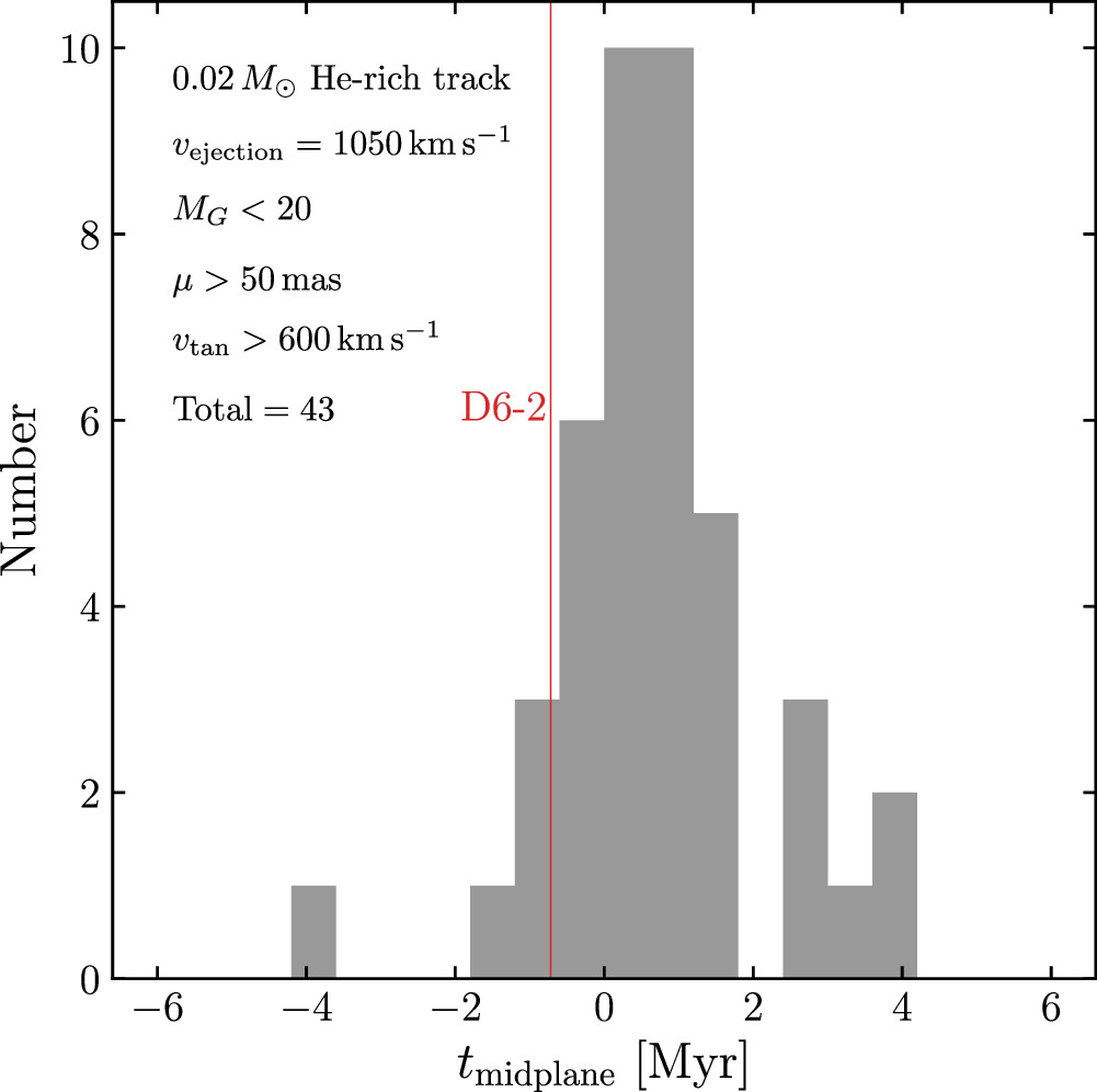
Figure 1: A histogram of detectable hyper-velocity survivors from the He-rich track assuming every Type Ia supernova produces a companion with a mass of 0.02 solar mass. These survivors are assumed to be ejected from their Type Ia supernovae at a velocity of 1,050 km/s, matching D6-2. The x-axis, tmidplane, describes the apparent travel time from the midplane of the simulation’s galaxy. A negative value means the survivor was observed before it passed through the plane. A total count of 43 hyper-velocity survivors from every Type Ia supernova yields an estimated survival rate of about 2%. [Shen 2025]
Choose Your Own (Stellar) Adventure
This article suggests different evolutionary paths for how binary white dwarfs might evolve. Depending on the properties of the merger, the system might do any of the following:
- Trigger nuclear reactions within the outer shell of the primary without detonating the primary’s core
- Become a normal Type Ia supernova
- Leave behind a hyper-velocity remnant
- Become a SN 2002es-like supernova, which is a fainter type of Type Ia supernova
There are lots of potential outcomes for these types of binaries, and hyper-velocity survivors indicate just a tiny fraction of a particular configuration of binary white dwarfs (see Fig. 2).
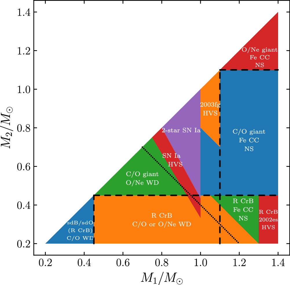
Figure 2: A diagram of the speculative outcomes for a white dwarf–white dwarf binary. The y-axis shows the secondary’s initial mass, whereas the x-axis shows the primary’s initial mass. The dashed lines indicate where the combined white dwarf mass is 1.4 M☉. The plot illustrates the wide variety of outcomes of white dwarf–white dwarf binaries, of which hyper-velocity survivors (HVS) are rare. sdB/sdO = subdwarf B/O stars; R CrB = R Coronae Borealis, variable star; Fe CC = iron core-collapse supernovae; HVS = hyper-velocity survivor; NS = neutron star. [Shen 2025]
Original astrobite edited by Chloe Klare.
About the author, Mckenzie Ferrari:
I’m currently a PhD grad student in the Geophysical Sciences program at the University of Chicago. While I now study the atmosphere and oceans of Earth, most of my previous undergrad and grad research focused on simulations of Type Ia supernovae and galaxy formation and evolution. In my free time, I foster cats for a local organization, enjoy cooking, and can often be found running along Lake Michigan.