Rapid Microlensing Classification: A Lonely SOBH Story
Editor’s Note: Astrobites is a graduate-student-run organization that digests astrophysical literature for undergraduate students. As part of the partnership between the AAS and astrobites, we occasionally repost astrobites content here at AAS Nova. We hope you enjoy this post from astrobites; the original can be viewed at astrobites.org.
Title: On Finding Black Holes in Photometric Microlensing Surveys
Authors: Zofia Kaczmarek et al.
First Author’s Institution: Lawrence Livermore National Laboratory; Heidelberg University
Status: Published in ApJ
Searching for stellar-mass black holes is no simple task — how do you look for an object floating in the vastness of space, hundreds or thousands of light-years away, that is at best the size of Houston, Texas, and emits no light? As our surveys of the night sky become more and more regular and increase in resolution, there is hope that we will be able to observe more and more chance alignments of these objects with stars, generating an observable effect known as microlensing. This mechanism provides us with a way to pick a proverbial black hole needle from the galactic stellar haystack, but the data we get from these surveys are still difficult to process efficiently. Today’s article introduces a new method for rapidly assessing the chances that a given microlensing event is indeed caused by a wandering black hole, allowing astronomers to make more effective decisions about which events to follow up on with targeted observation campaigns.
A Microlensing SOBH Story
While astrophysical black holes were once squarely in the realm of speculative science fiction, it is now commonplace to find these extreme objects through a variety of techniques. One such technique involves observing a star that is moving around in a binary system, making its motion regular and predictable. Astronomers can use this regular motion to deduce the mass of the star’s partner — and if there’s no visible signal associated with the companion, it may turn out to be a black hole.
Another more recent technique that has proven successful in finding these exotic objects involves listening for the gravitational waves produced when a black hole merges with another compact object like a black hole, neutron star, or white dwarf. From these observations, astronomers can learn about the overall population of black holes in our universe, and by proxy can learn about the last stages of stellar evolution. But relying on these measurements alone would generate a biased picture of stellar evolution, because they only pick out black holes that formed in (or evolved into) binary systems. This leaves us without much information about the non-negligible fraction of stars (and therefore black holes) that prefer the “single life.”
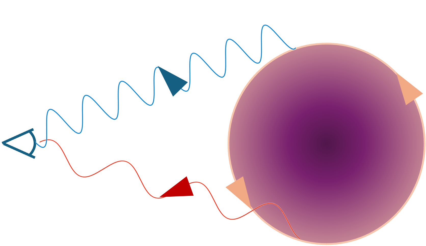
Figure 1: Cartoon depiction of the process of gravitational microlensing. A foreground object intersecting our line of sight to a bright background object can cause optical distortions like brightening and doubled images. [NASA Ames/JPL-Caltech/T. Pyle]
One Quick Classification Trick
For the most part, microlensing events are found by looking for subtle changes in the light coming from a star — this observation is a photometric measurement of the microlensing event. Photometric data for a microlensing event are generally able to provide at least some constraints on two important microlensing parameters: the Einstein timescale 𝑡𝐸 (related to how long the foreground object lenses the background as it passes by) and the microlensing parallax 𝜋𝐸, which results from Earth’s acceleration towards or away from a particular lensing event. Unfortunately, from these variables alone it can be hard to confidently determine the nature of the lensing object, motivating attempts to make higher-resolution follow-up observations of these events. Telescopes with strong spatial resolution can sometimes pick up on the way the lensing object subtly distorts the apparent position of the background star. These so-called astrometric observations can help pin down important information such as the size and/or mass of the lensing object, letting astronomers confirm the presence of a SOBH or another object of interest.
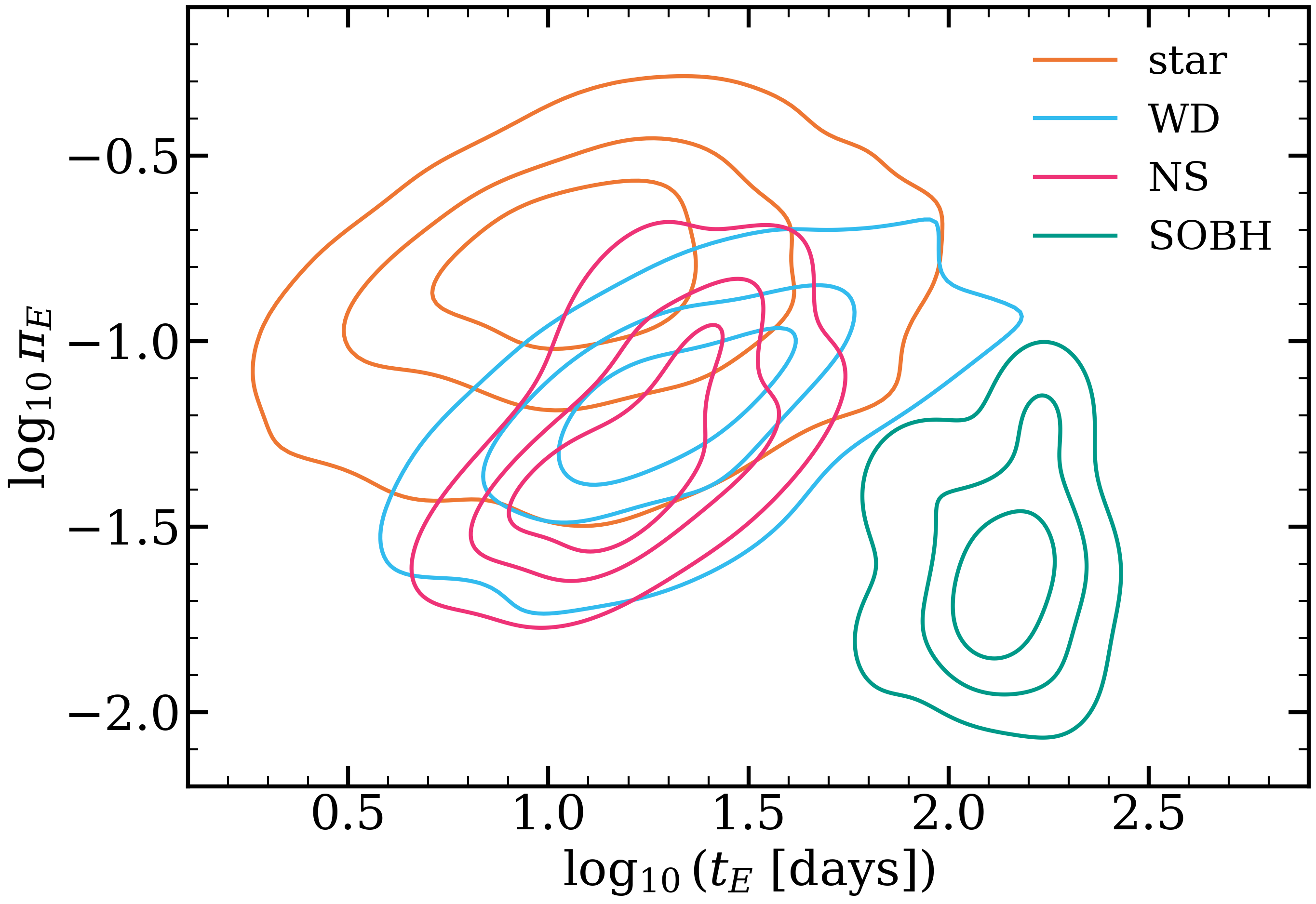
Figure 2: This plot from today’s article shows the distribution of two microlensing parameters produced by various lensing sources. The separation of SOBHs in this parameter space indicates that measurement of these parameters in photometric data may allow for the rapid identification of microlensing events caused by SOBHs. [Kaczmarek et al. 2025]
After introducing their classification pipeline, the authors applied it to an existing microlensing dataset from the OGLE collaboration. This dataset contained nearly 10,000 events, from which the classification pipeline returned 23 high-probability SOBH candidates that were agreed upon across all three models of star-to-black-hole evolution (“initial–final mass relations”) the authors used. Applying further selection rules to find candidate events that could potentially be observed by the Gaia telescope, the list was whittled down to just four events. Unfortunately, all four of these remaining candidates were found to be unlikely to produce significant astrometric deviations, meaning we will likely have to wait for larger microlensing surveys coming up in the near future for a solid chance of finding a new SOBH candidate with this method.

Figure 3: This plot from today’s article depicts the estimated 𝑡𝐸 and 𝜋𝐸 parameters for the only confirmed SOBH microlensing event compared against the regions of parameter space expected to correspond to white dwarfs (blue) and SOBHs (green). The minimal overlap with the green region indicates that this event may have been an outlier compared to galactic stellar population models. [Kaczmarek et al. 2025]
OB110462: A Chance Encounter?
Using a stellar-population-model-informed classification method like the one presented in this article may also allow us to directly examine weaknesses in these models. For example, if in the future we find many microlensing events that are later confirmed to be SOBHs but exist outside of the expected SOBH region of 𝑡𝐸–𝜋𝐸 parameter space, it could point us towards a flaw in the underlying population models. As of the publication of this article, however, we only have one confirmed SOBH microlensing event to compare to (denoted OB110462). Working with a sample size of one is pretty uninformative (to say the least), but the authors do note that this event is already somewhat of an outlier given their population model. In Figure 3, you can see the recovered 𝑡𝐸 and 𝜋𝐸 probability contour for OB110462 only barely overlaps with the region corresponding to SOBHs, and the contours fit more snugly in the region corresponding to white dwarfs. This tension is interesting, because even if it doesn’t point to a problem with the stellar population models, it could indicate that the successful confirmation of this event as a SOBH was an unlikely success, and so choosing to dedicate time on Hubble to do follow-up measurements was, in retrospect, a high-risk move that paid off.
Regardless of how things turned out with OB110462, this sort of analysis points to a more general benefit this classification scheme provides: it allows for a very rapid estimation of which microlensing events we should focus our attention on with follow-up observations. The authors propose that this makes their method ideally suited as an initial filter through which microlensing events can pass before more complicated analyses are performed. As surveys like the Vera C. Rubin Observatory Legacy Survey of Space and Time begin to take unfathomably huge amounts of time-domain data, the number of detected microlensing events is going to sharply increase, making it more important than ever that we think carefully about which events are worth following up on.
Original astrobite edited by Lindsey Gordon.
About the author, Lucas Brown:
I’m a graduate student at the University of California, Santa Cruz. My research involves figuring out how to use exotic phenomena like gravitational waves to learn about elusive astrophysical objects like primordial black holes or dark matter. Outside of physics I love playing piano, climbing, and spending time with my dog.

 Breaks")