?")
What if Mars Were a Stranger (Thing)?
Editor’s Note: Astrobites is a graduate-student-run organization that digests astrophysical literature for undergraduate students. As part of the partnership between the AAS and astrobites, we occasionally repost astrobites content here at AAS Nova. We hope you enjoy this post from astrobites; the original can be viewed at astrobites.org.
Title: Mars as an Exoplanet: Lessons from a Planet at the Edge of Habitability
Authors: Stephen R. Kane et al.
First Author’s Institution: University of California, Riverside
Status: Published in PSJ
Mars in the Upside Down
If you’re a fan of Stranger Things like me, you’ll know of the Upside Down: a mirror world similar to our own, but with very different rules. Imagine Mars in the Upside Down, where it is no longer our next-door neighbor but a planet hundreds of light-years away. An astronomer on this Upside Down Earth would be looking at a distant speck with a transit signal barely distinguishable from noise. In this world, Mars would no longer be familiar but completely foreign, with unknown properties. Kane et al. suggest that treating Mars as if it were a stranger is a useful way to think about exoplanet science today.
JWST is hunting for atmospheres on small rocky planets around other stars. However, only a select few Mars-like exoplanets have been discovered (Figure 1). This is because sub-Earth planets are small and hard to detect, testing the bounds of current technology. The ones that have been discovered, such as TRAPPIST-1h and Kepler-138b, were detected due to favorable geometry. They happen to orbit very close to a low-mass star or sit in resonant multi-planet systems, which amplify the signal we are looking for. True Mars analogs with low flux and moderate orbital periods remain out of reach. This is precisely what makes Mars itself so important scientifically — it is the only planet of this type we can study up close.
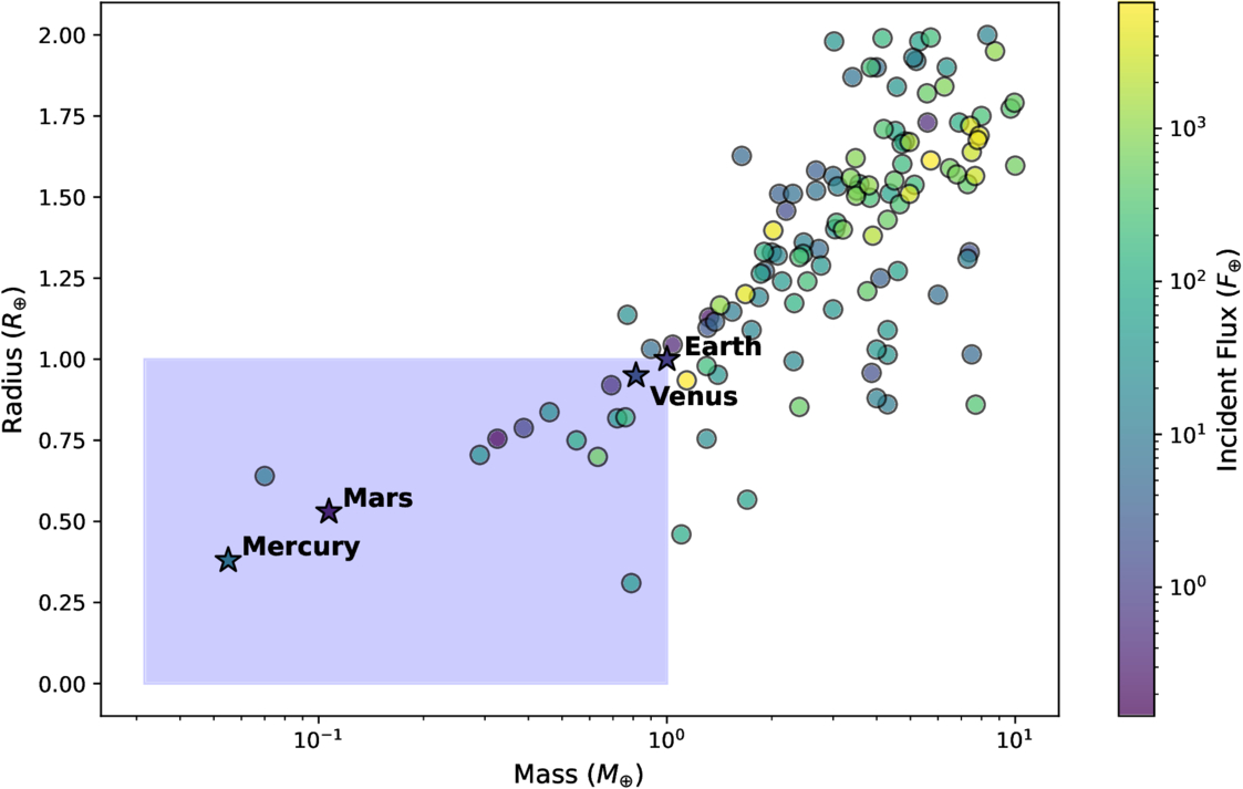
Figure 1: A plot of confirmed exoplanets by mass and radius. Most confirmed exoplanets are larger and more massive than Earth. Mars-like planets (dots in the blue box) are rare in confirmed exoplanet detections. [Kane et al. 2026]
Getting to Know Mars, Getting to Know All About Mars
We know a lot about Mars in comparison to other planets thanks to rovers (such as Curiosity and Perseverance), atmospheric orbiters (such as Mars Atmosphere and Volatile EvolutioN and the Mars Orbiter Mission), and other science missions (Figure 2). We know it once had water features with neutral pH and favorable chemistry for life from sedimentary evidence at the Gale and Jezero craters. We know its atmosphere is 95% CO2 with a surface pressure less than 1% of Earth’s. We know it once had an active magnetic dynamo, but the dynamo died out about 4 billion years ago, leading to solar wind steadily stripping away Mars’s atmosphere over time.
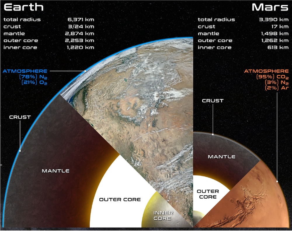
Figure 2: Earth and Mars to scale, showing their internal structures and atmospheres. Despite being neighbors, Mars is dramatically smaller with a thin CO2 atmosphere, similar to the planets JWST is struggling to characterize. [Kane et al. 2026]
Beyond Our Backyard
JWST is currently studying the small rocky TRAPPIST-1 planets and is finding little evidence of atmospheres. The authors of today’s article explore the idea that these exoplanets are similar to Mars and perhaps are undergoing processes that strip away their atmospheres and create optimal conditions for life only for short durations. Using Mars as a blueprint, the authors show how we can better understand exoplanet processes, including volatile delivery and loss, photochemistry, climate evolution, obliquity forcing, planetary architecture, and intrinsic magnetism. For example, measurements of noble gases directly fingerprint Mars’s atmospheric escape process, and the authors argue these give us a calibration framework for interpreting future exoplanet spectra.
The upcoming Nancy Grace Roman Space Telescope’s microlensing survey will start revealing how common true Mars analogs actually are throughout the galaxy, while the future Habitable Worlds Observatory will attempt direct imaging of nearby candidates with unprecedented precision. Together, these missions will tell us whether Mars-like outcomes (brief habitability, catastrophic atmospheric loss, barren surfaces, etc.) are the default fate for small rocky planets. Interpreting that data will require the exact framework this article builds: one grounded in the only Mars analog we can study in detail.
Original astrobite edited by Sandy Chiu.
About the author, Ben Sherwin:
I am a physics PhD student and a National Science Foundation Graduate Research Fellow at Stanford University, working with Josh Frieman. I am interested in theoretical and observational cosmology, specifically in cross-correlations between the cosmic microwave background and tracers of large-scale structure.


 Edge")

