Features RSS

Image of two bright blue stars side by side and one dimmer circled star below, against a background of more distant stars.

Editor’s note: In these last two weeks of 2018, we’ll be looking at a few selections that we haven’t yet discussed on AAS Nova from among the most-downloaded papers published in AAS journals this year. The usual posting schedule will resume in January.

Alpha Centauri Beyond the Crossroads

Published January 2018

Main takeaway:

A scientist from University of Colorado Boulder, Tom Ayres, has compiled observations from the Chandra X-ray Observatory tracking the X-ray emission from the two stars of the Alpha Centauri binary system. Alpha Centauri is the closest star system to us, at just 4.37 light-years away.

Why it’s interesting:

Alpha Centauri A and B are both Sun-like dwarf stars with coronae very similar to our Sun’s. By studying the X-ray activity of these stars, we can learn more about how stars like the Sun bombard their environments with harsh radiation. This is useful both from the perspective of protecting our own interests — since this so-called space weather can affect astronauts, satellites, our power grid, etc. — and from the perspective of learning about potential habitability around our nearby stellar neighbors.

On Alpha Centauri’s recent crossroads:

X-ray light curves

X-ray light curves of Alpha Centauri A (blue), Alpha Centauri B (red), and the Sun (gray) for 1995–2018. [Ayres 2018]

The latest Chandra observations are cool because we can distinctly see the stellar activity cycles in both Alpha Centauri A and B, in much the same way that our own Sun has an 11-year cycle. For Alpha Centauri B, the cycle is about 8 years; for Alpha Centauri A, it appears to be closer to 19 years. In 2016, the system reached what Ayres describes as a crossroads: not only did Alpha Centauri A hit a maximum in activity and Alpha Centauri B hit a minimum, but around the same time, we also witnessed the crossing of the apparent trajectories of the two stars on the sky.

Citation

T. R. Ayres 2018 Res. Notes AAS 2 17. doi:10.3847/2515-5172/aaa88f

GW170817

Just last year, the three observatories of the Laser Interferometer Gravitational-Wave Observatory (LIGO)–Virgo Collaboration detected the gravitational-wave signature of two neutron stars colliding. What can we learn from the months of observations made since?

GW170817 signal

On 17 August, 2017, LIGO detected this “chirp” as two neutron stars spiraled inward and collided. This brief gravitational-wave blip, known as GW170817, has been followed up with months of multiwavelength observations. [LSC/Alex Nitz]

When Worlds Collide

Immediately following the detection of gravitational-wave event GW170817, teams of astronomers around the world rushed to pinpoint and characterize the electromagnetic radiation from the source.

These early observations were hugely important for validating our understanding of what happens when neutron stars collide, but the work didn’t end there; in the months that followed, repeated measurements of the flux across the electromagnetic spectrum have provided us with the tools to probe what happened in the aftermath of the merger.

These late-time observations should allow us to distinguish between two competing post-merger scenarios, in which the resultant relativistic jet either pushes past the previously ejected material surrounding the remnant (the “jet-dominated outflow” model) or fails to escape the slow-moving shroud of material (the “cocoon-dominated outflow” model) and is choked.

Mooley et al. 2018 Fig. 1

Radio spectral indices from 6 to 10 months post merger. Combining all the radio data gives a spectral index of -0.53. The black line shown for reference is the radio-to-X-ray spectral index measurement. [Mooley et al. 2018]

Tuning in to GW170817

In order to characterize the nature of the outflow and determine which scenario describes GW170817, a team led by Kunal Mooley (National Radio Astronomy Observatory/Caltech) analyzed the decline of GW170817’s radio emission over time. The authors combined data from multiple radio sources — MeerKAT, Very Large Array (VLA), Giant Metrewave Radio Telescope (uGMRT), and the Australia Telescope Compact Array (ATCA) — to cover the radio emission from 0.65 to 12 GHz.

After steadily rising for 5–6 months after the event, the radio emission peaked and quickly began to decline, making the transition from rising to falling in just a few weeks. The authors focused on two important features of the radio light curve: how rapidly the flux density decreases after the peak (the power-law decay index) and how “sharp” the peak of the light curve is.

Mooley et al. 2018 Fig. 2

Radio data used in this study. All measurements have been scaled to 3 GHz. The black line is the best-fit model. [Mooley et al. 2018]

Jet vs. Cocoon

Models tell us that if GW170817’s jet were choked by a slow-moving cocoon of material, the radio observations would reveal a power-law decay index of -0.88. If instead the jet punches free of the material as in the jet-dominated outflow model, its flux density would decrease much more rapidly, exhibiting a power-law decay index of -2.17.
So which model do the radio observations of GW170817 support? All of the post-peak data are well-described by a single power-law decay with an index of -2.4. This strongly supports the jet model over the cocoon model, and it suggests that the majority of the energy in the post-merger outflow is carried away by the jet.

The sharpness of the light-curve peak is dependent upon the viewing angle and the width of the jet. Based on a simple jet model, the authors find that the jet is likely very narrow (with an opening angle of less than 10°) and the viewing angle is less than 28°. Future modeling will explore the effects that structure in the jet can have on how sharply peaked the radio light curve is and further our understanding of these highly energetic collisions.

Citation

“A Strong Jet Signature in the Late-time Light Curve of GW170817,” K. P. Mooley et al 2018 ApJL 868 L11. doi:10.3847/2041-8213/aaeda7

TESS first light

How do we find the signals of exoplanets lurking in the vast quantity of data that comes out of a mission like Kepler or the Transiting Exoplanet Survey Satellite (TESS)? A new study has some suggestions for how best to get computers to do the heavy lifting for us.

Managing a Mess of Data

false positives

Two common false positives — grazing eclipsing binaries (left) and background eclipsing binaries (right) — can mimic the signal of a transiting planet. [NASA/Ames Research Center]

Recent years have seen a boom in exoplanet research — in large part due to the enormous data sets produced by transiting exoplanet missions like Kepler and, now, TESS. But the >3,000 confirmed Kepler planets weren’t all just magically apparent in the data! Instead, the discovery of planets is the result of careful classification of transit-like signals amid a sea of false positives from things like stellar eclipses and instrumental noise.

Given the number of light curves that need classifying, we can use any automated help we can get. Enter machine learning, a process by which computers can be trained to identify patterns and make decisions. Using a tool called deep learning, scientists have already shown that machines can do a pretty good job of automatically classifying Kepler transit signals as either exoplanets or false positives. But can we do even better?

light curves and centroids

Local (left) and global (right) views of the light curves (cyan) and centroids (maroon) for an example confirmed planet (top) and background eclipsing binary (bottom). Click for a closer look. [Ansdell et al. 2018]

The recent 2018 NASA Frontier Development Lab provided an excellent opportunity to find out. This eight-week research incubator was aimed at applying cutting-edge machine-learning algorithms to challenges in the space sciences. As part of this lab, two machine-learning experts were paired with two space-science researchers to try to improve machine-learning models for exoplanet transit classification. The results are presented in a new publication led by scientist Megan Ansdell (Center for Integrative Planetary Science, UC Berkeley).

Insider Knowledge

Ansdell and collaborators started with a basic machine-learning model that classified signals based on straightforward local and global views of the light curves. To improve upon it, they added scientific domain knowledge — information or insight that might not be generally known, but can be provided by a domain expert. 

Exonet recall and precision

Recall (top; the fraction of true planets recovered) and precision (bottom; the fraction of classifications that are correct) of the Exonet model, as a function of MES, a measure of the signal-to-noise of candidate transits. [Ansdell et al. 2018]

In particular, the authors used their knowledge of what types of false positives might come up. To help distinguish background eclipsing binary stars from planet transit signals, the team included data with each light curve showing how the line centroids — the pixel positions of the center of light — moved over time. To help the model identify false positives like giant-star eclipsing binaries, the authors fed in known stellar parameters with the light curves.

More Planets to Come

How did Ansdell and collaborators do? Using their modified model, “Exonet”, a computer can classify a Kepler data set with 97.5% accuracy and 98% average precision. That means that 97.5% of its classifications — exoplanet or false-positive — are correct, and an average of 98% of transits classified as planets are true planets. Not bad, for a machine!

One of the added benefits of the authors’ model is that it is ideal for generalization — for example, from Kepler to TESS data. The authors are currently working on a study using Exonet to classify simulated TESS data. And yesterday’s first public data release from TESS has provided plenty of fresh data to work with in the future!

Citation

“Scientific Domain Knowledge Improves Exoplanet Transit Classification with Deep Learning,” Megan Ansdell et al 2018 ApJL 869 L7. doi:10.3847/2041-8213/aaf23b

SDO/AIA 193

How is energy released in explosive events like flares and jets? One of the most likely culprits is magnetic reconnection — but we still have a lot of questions about how this process works. In a recent study, radio observations of the Sun provide us with a closer look.

A Nearby Laboratory

reconnection point

Observations of radio bursts allow the authors to trace the trajectories of electron beams (colored points and tracks) back to their common reconnection sites (marked by stars). Two different groups of beams are shown in (a) and (b). Background is the SDO/AIA 193 Å EUV image. [Adapted from Chen et al. 2018]

Fast magnetic reconnection is a plasma process in which magnetic field lines with opposite directions approach each other and then abruptly reconfigure. According to theory, the suddenly released magnetic energy can then be converted, heating the surrounding plasma and accelerating particles like electrons to semirelativistic speeds.

Unfortunately, testing this model against observations poses a challenge: most astrophysical jets — like those at the centers of active galaxies — lie vast distances away from us, preventing us from exploring the process of reconnection in detail. Thus, questions like where and how electrons get energized are difficult to answer, since we can’t easily observe the process.

There is one convenient nearby laboratory in which we can study reconnection, however: the Sun. In a new study, a team of scientists led by Bin Chen (New Jersey Institute of Technology) have used high-resolution radio observations of the Sun to pinpoint the location of magnetic reconnection and particle acceleration with greater accuracy than ever before.

Pinpointing Acceleration

Chen and collaborators used the unique capabilities of the Karl G. Jansky Very Large Array (VLA) to observe bursts of radio emission associated with a solar jet in November 2014. Radio bursts like these are emitted from groups of electrons that travel along tubes of magnetic flux at incredible speeds — between one tenth and one half the speed of light! By observing these radio bursts, the authors hoped to answer a fundamental question: where exactly did the emitting electrons first get accelerated?

magnetic modeling

Three-dimensional magnetic model of the jet eruption — during pre-eruption (left), rise (center), and eruption (right) phase — from the perspective of an observer at Earth (top) and as viewed from the side (bottom). The stars indicate the origins of the electron beams and sites of reconnection. Click to enlarge. [Chen et al. 2018]

By combining their radio observations with extreme ultraviolet imaging from the Solar Dynamics Observatory (SDO), X-ray data from the Reuven Ramaty High Energy Solar Spectroscopic Imager (RHESSI), and three-dimensional magnetic modeling, the authors are able to trace the origin of each group of electrons back to an extremely compact region in the low solar corona.

This unprecedented localization of the electrons’ source to an area of just ~600 km2 allows Chen and collaborators to conclude that this location is a magnetic reconnection null point — a central location where different magnetic flux tubes are brought together, reconfigure, and release magnetic energy, accelerating electrons during a brief (less than 50 milliseconds!) reconnection event behind the erupting jet spire.

Chen and collaborators demonstrate that these unprecedented observations provide new constraints for magnetic reconnection models, bringing us one step closer to understanding the explosive releases of energy from magnetic structures in our universe.

Citation

“Magnetic Reconnection Null Points as the Origin of Semirelativistic Electron Beams in a Solar Jet,” Bin Chen et al 2018 ApJ 866 62. doi:10.3847/1538-4357/aadb89

HAT-P-11b

The atmospheres of planets close to their host stars live a tenuous existence. New observations from the Hubble Space Telescope show signs of a Neptune-like exoplanet’s atmosphere being eroded away.

Evaporation at Work

Small planets observed to orbit closely around their host star fall into two main populations:

  1. those with radii smaller than 1.5 Earth radii, thought to be primarily rocky cores with little or no remaining atmosphere, and
  2. those with radii larger than 2 Earth radii, thought to retain some of their hydrogen and helium atmospheres.

What causes the difference between these two populations? We think that all close-in exoplanets are sculpted by the energetic radiation of their host stars. This radiation can erode away the primordial atmospheres — and for the smallest planets, this will leave only their rocky cores behind.

As we work to understand the detailed physics of this photoevaporation, it would be helpful to be able to directly watch a planet’s atmosphere escaping in this way. In a new study, scientist Megan Mansfield (University of Chicago) and collaborators present just the thing: observations of the escaping atmosphere of the exoplanet HAT-P-11b.

Observations of a Hot Neptune

WASP-107b

Artist’s illustration of WASP-107b, the first planet for which Hubble discovered helium escaping from its atmosphere. [ESA/Hubble, NASA, M. Kornmesser]

HAT-P-11b is a Neptune-sized exoplanet that orbits very close to its host star in a system that’s located approximately 120 light-years from Earth. Using Hubble, Mansfield and collaborators discovered the subtle signature of helium escaping from the atmosphere of HAT-P-11b — making this the second planet for which this signature has been discovered by Hubble (the first was WASP 107-b) and one of only a handful of planets for which we’ve seen signs of atmospheric escape.

By comparing these observations to models, Mansfield and collaborators estimate that HAT-P-11b is losing mass at a rate of roughly 109–1011 g/s. This rate, while high, is still low enough that the planet has only lost a few percent of its mass over its history, leaving its bulk composition largely unaffected. This is consistent with what we would expect for a planet of its size: since it’s larger than 2 Earth radii, it should retain some of its hydrogen and helium atmosphere.

Narrowband spectrum of HAT-P-11b

Narrowband spectrum of HAT-P-11b (blue and gray points) compared to three 1D models of hydrodynamic escape (red, green, and orange lines). [Mansfield et al. 2018]

A New Approach

Why are these escaping-helium detections important? Observations like this one represent a new method for exploring exoplanet atmospheres! The helium signature detected from HAT-P-11b had long been theorized as a way to study escaping atmospheres, but until Hubble’s recent observations of helium in the atmosphere of WASP 107-b, the potential of this approach remained untapped.

Now two planets have been observed with this particular signal — and the signal from HAT-P-11b has been additionally confirmed with CARMENES instrument in Spain, marking the first time the same signature of photoevaporation has been detected by both ground- and space-based facilities.

Future observations like these — from both existing instruments and upcoming observatories like the James Webb Space Telescope — will hopefully continue to shed light on how atmospheres evaporate from small, close-in exoplanets.

Citation

“Detection of Helium in the Atmosphere of the Exo-Neptune HAT-P-11b,” Megan Mansfield et al 2018 ApJL 868 L34. doi:10.3847/2041-8213/aaf166

Very Large Array (VLA)

Humanity’s search for signs of extraterrestrial intelligence has been underway, in one form or another, for decades. But how much searching have we really done?

Green Bank Telescope

The 100-meter Green Bank Telescope has been used to search for radio signals from extraterrestrial civilizations. It was also used to eavesdrop on signals from interstellar asteroid ‘Oumuamua in 2017. [NRAO/AUI/NSF]

Where Is Everybody?

With the number of known potentially habitable exoplanets increasing every day, it’s easy to feel both optimistic about and overwhelmed by our chances of finding life on other planets. The search for life elsewhere in the universe has led astronomers to carry out highly precise observations of exoplanet atmospheres in the hopes of detecting biosignatures — like the subtle imprint that gaseous oxygen and methane would leave on an exoplanetary spectrum.

The search for extraterrestrial intelligence (SETI), on the other hand, looks for technosignatures rather than biosignatures. Technosignatures could take many forms, like the excess waste heat emitted by structures designed to harness the energy of a star, but most SETI efforts focus on extraterrestrial radio signals. For all our decades of searching, we’ve yet to find any convincing signals, leading some to believe that there are no signals to be found.

Have we truly plumbed the depths of the cosmic ocean and come up empty-handed, meaning that we should abandon our search? To answer this question, a team led by Jason Wright (The Pennsylvania State University) devised a way to calculate how much of the available parameter space we’ve really searched.

Wright, Kanodia & Lubar Table 1

The boundaries for the example haystack used in this work. Click to enlarge. [Wright, Kanodia & Lubar 2018]

Measuring n-dimensional Volumes

Wright and collaborators based their calculations on a concept called the cosmic haystack: a volume containing naturally occurring radio signals and (hopefully!) at least one artificial signal from an intelligent extraterrestrial civilization — the proverbial needle that rounds out the metaphor.

But quantifying our progress in the search for extraterrestrial intelligence is more complicated than just considering the fraction of the sky we’ve observed; the spatial volume surveyed is just one of the many dimensions of the cosmic haystack. Just as observing only a few stars would greatly limit the physical volume of your survey, only searching for signals in a narrow frequency range limits yet another dimension of the cosmic haystack.

In addition to the spatial volume, Wright and collaborators also included the sensitivity of the survey, the bandwidth, polarization, and modulation of the signal, and the repetition rate, as dimensions of the haystack. This makes for a searchable haystack with no fewer than nine dimensions! Based on reasonable search parameters, the authors estimate the total volume of the cosmic haystack to be 6.4 × 10116 m5 Hz2 s W-1.

More Than a Drop in the Bucket?

Of that immense volume, we’ve searched a mere 2.4 × 1098 m5 Hz2 s W-1, which amounts to a fraction of 3.8 × 10⁻¹⁹. This is equivalent to a small swimming pool’s worth of water compared to the volume of Earth’s oceans!

Feeling discouraged that after decades of listening, we’ve really only just begun our search? Carefully designed surveys — like those with wide fields of view that make repeated observations of each patch of sky — have the potential to quickly scour large swaths of the cosmic haystack. Hopefully, there are plenty of needles to be found.

Citation

“How Much SETI Has Been Done? Finding Needles in the n-dimensional Cosmic Haystack,” Jason T. Wright, Shubham Kanodia, and Emily Lubar 2018 AJ 156 260. doi:10.3847/1538-3881/aae099


WFIRST

New exoplanets, distant galaxies, unexpected transients — the successful discoveries of major astronomical missions get splashed across news headlines. What generally isn’t seen, however, is the often decades-long development process that led to these successful missions — a process that includes not only technology and engineering feats, but also the meticulous planning necessary to optimize the use of an observatory with a limited lifetime.

Want a closer look? A recently published study provides an insider’s view of these complex planning stages for a proposed upcoming mission, the Wide Field Infrared Survey Telescope (WFIRST).

A New Eye in the Sky

dark energy

Schematic of the expansion of the universe. WFIRST would use supernovae to learn more about the nature of dark energy. [NASA/WMAP]

In 2010, the astronomy community selected WFIRST as the highest-ranked large space-based mission for the next decade. Like most major missions, WFIRST has been through its share of ups, downs, and funding scares in the planning process — but as of this writing, it’s on the books for a planned launch in the mid 2020s.

WFIRST will use a telescope the size of Hubble’s (i.e., a 2.37-m mirror) that was donated in 2012 by the National Reconnaissance Office. It will host two main instruments: a coronagraph that will be used for exoplanet and planetary disk studies, and a wide-field instrument that will be used to probe dark-energy models. The wide-field instrument will have two components: a wide-field channel imager, and an integral field channel spectrometer. 

Vying for Time

Looking at just the dark-energy science objective, we can already see timing challenges emerge. WFIRST seeks to constrain the nature of dark energy by discovering and measuring the distance to Type Ia supernovae, thereby measuring the evolution of dark energy over time.

survey strategies

Comparison of the predicted range of values for the figure of merit (FoM) number — a metric that characterizes how well we understand the dark-energy equation of state — for different survey strategies. Spectrometer-focused strategies are shown in the top panel, and imager-focused strategies are shown in the bottom panel. The red dashed line indicates our current level of understanding. [Hounsell et al. 2018]

But though WFIRST’s proposed mission duration is five years, only a total of 6 months of observing time can be devoted to the supernova survey. Should this time be primarily spent on wide-field imaging to detect as many supernovae as possible? Or should we employ a targeted strategy, using the spectrometer to better determine redshifts of the supernovae discovered? What areas should the survey cover, at what depth? How frequently should we look at the same patches of sky?

These are just some of the many questions survey designers must wrestle with in order to optimize the WFIRST mission and give the project the best chance of answering our questions. To aid decision-making, a team of scientists led by Rebekah Hounsell (University of California, Santa Cruz and University of Illinois at Urbana-Champaign) has now conducted a series of simulations to explore different supernova survey strategies for WFIRST.

An Optimized Reference

dark-energy equation of state parameters

Example confidence contours for our knowledge of two parameters that describe the dark-energy equation of state and its evolution over time, for some of the survey strategies the authors propose. All the survey strategies provide significant improvement over our understanding from just cosmic-microwave-background and baryon-acoustic-oscillation constraints (shown in blue for comparison). [Adapted from Hounsell et al. 2018]

Hounsell and collaborators realistically simulated supernova light curves and spectra as viewed by WFIRST’s instruments. They then explored 11 survey strategies with different time allocations between the imager and the spectrometer, taking into account various uncertainties. Their results suggest an imaging-focused strategy would be the most successful at increasing our understanding of the dark-energy equation of state.

Though we won’t know exactly which strategy is the most optimal until we’ve determined some of the specific systematic uncertainties of the mission, Hounsell and collaborators’ study has laid the groundwork for future planning of the mission. What’s more, their results confirm that WFIRST will have the potential to significantly advance our understanding of dark energy — so keep an eye on this project in the future!

Citation

“Simulations of the WFIRST Supernova Survey and Forecasts of Cosmological Constraints,” R. Hounsell et al 2018 ApJ 867 23. doi:10.3847/1538-4357/aac08b

In March of this year, a team of scientists announced an unprecedented radio detection: a signal from the first stars that formed in the universe. But the shape of this signal was not quite what we predicted — and theorists are now exploring what this means about the dawn of the universe.

A Cosmic Timeline

cosmic timeline

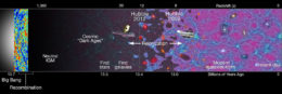
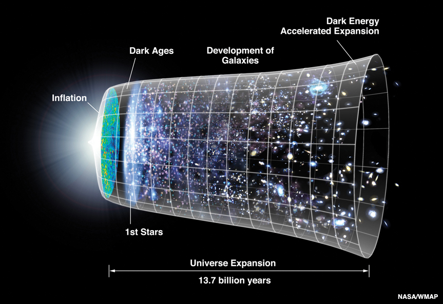
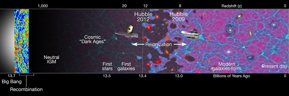
Timeline showing the evolution of the universe since the Big Bang. Click to enlarge. [NASA/ESA]

Our models of cosmic history tell us that after the Big Bang, the expanding universe consisted of a hot, opaque, ionized soup of gas. Perhaps 370,000 years later, recombination of these electrons and protons into neutral hydrogen atoms allowed light to travel freely through the universe — releasing the radiation we see today as the cosmic microwave background (CMB).

At this stage in the universe’s history, there were not yet any stars or galaxies. With no sources of light, the universe continued on in the “cosmic dark ages” until redshifts of around z ~ 20, perhaps 100–200 million years after the Big Bang. By then, dark matter and gas had clumped into bound objects dense enough to ignite nuclear fusion — lighting up the first stars of our universe.

absorption feature

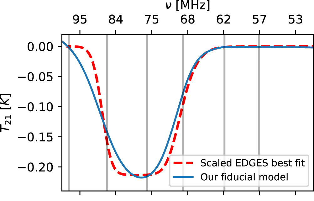
The shape of the best-fit EDGES signal is shown in the red dashed line; the corresponding signal from the authors’ model, in which the first stars are preferentially clustered in halos with mass above 10^9.4 solar masses, is shown with a blue line. The authors’ goal here is only to reproduce the sharpness of the drop on the low-frequency (right) side of the signal. [Adapted from Kaurov et al. 2018]

Fingerprint of the First Stars

These first stars are very distant and faint, so we don’t yet have the technology to detect them directly. But the ultraviolet radiation that these hot, young stars emitted would have heated the gas around them. According to models, this hot gas would then have absorbed some of the background radiation, causing a small dip in the intensity of the CMB at the radio wavelengths of 21 cm.

It is this dip — this subtle fingerprint of the first stars — that the EDGES team detected. But the shape of the signal wasn’t exactly as we were expecting: it’s both significantly deeper and has much sharper boundaries than predicted.

While many studies have since been published attempting to explain the surprising depth of the signal, a team of scientists led by Alexander Kaurov (Institute for Advanced Study) has instead opted to focus on the other puzzle: that of the signal’s sharp boundaries.

early universe simulation

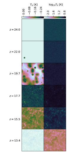
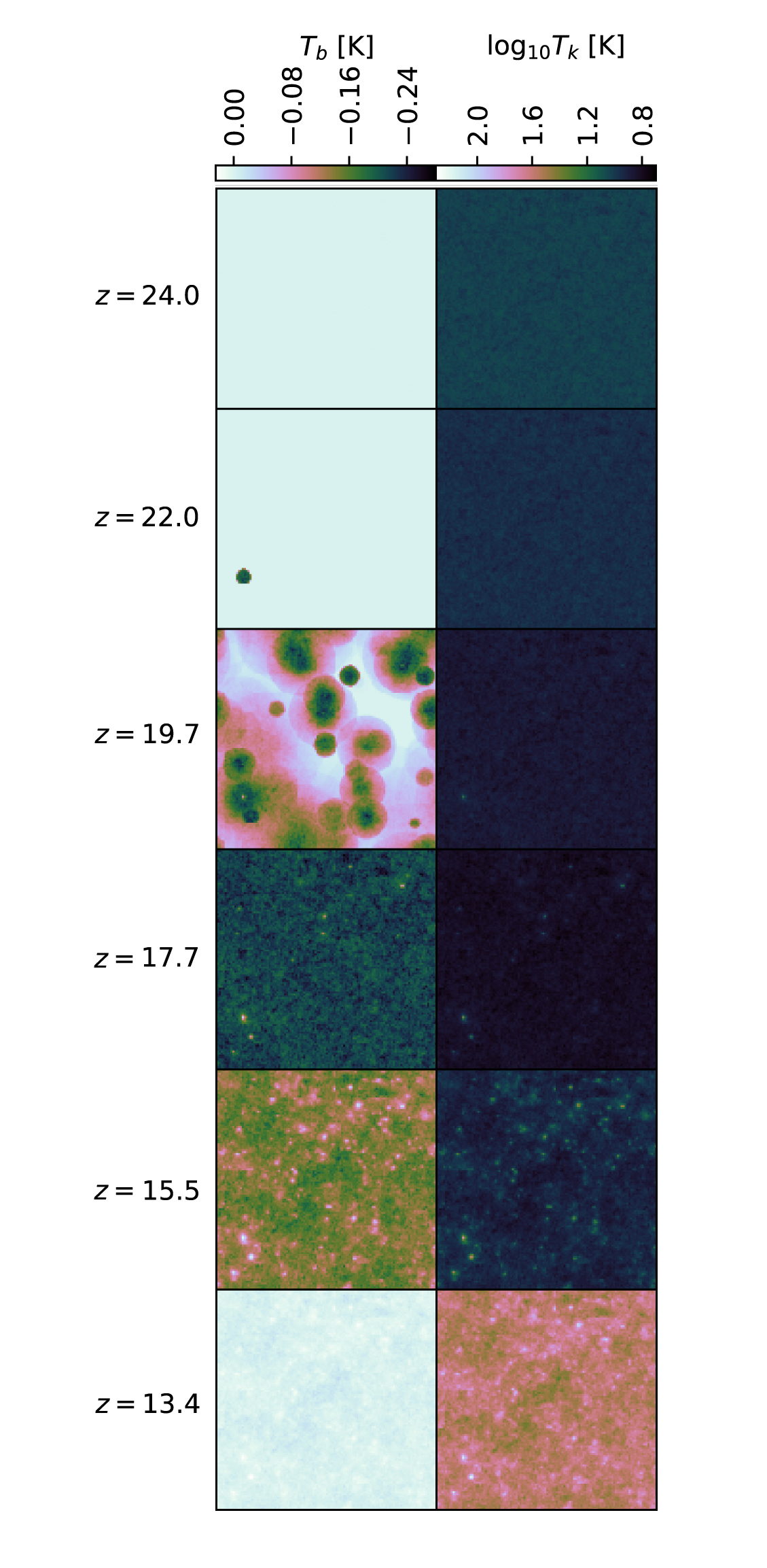
Inhomogeneous brightness temperature (left) and kinetic gas temperature (right) in the authors’ simulation, at six characteristic epochs. At ~ 24 no sources have formed yet; around ~ 22, evidence of the first sources is seen; by ~ 19.7, many more are present. [Kaurov et al. 2018]

Seeing the Light

In a recent publication, Kaurov and collaborators examined possible scenarios that could lead to the sharpness seen on the low-frequency side of the EDGES signal. Physically, this feature tells us that as the first stars turned on, the universe was flooded with ultraviolet photons much more quickly than we expected.

Kaurov and collaborators show that this suddenness can be naturally explained if the sources of these photons — the first stars — were not distributed evenly throughout the universe’s structure, but were instead initially concentrated only in the rarest and most massive halos — those weighing more than a billion solar masses.

Early in the universe, the number of these rare halos grew rapidly. The authors use simulations to confirm that this sudden explosion of massive halos hosting bright, hot stars could have produced the flood of ultraviolet photons necessary to explain the EDGES signal. 

If this scenario is correct, it has interesting implications for future observations. If the majority of the first stars were, indeed, located within the few rarest of halos, these halos would be especially bright. Though they’re scarce, these sources might be observable with the upcoming James Webb Space Telescope — providing us with another window into cosmic dawn.

Citation

“Implication of the Shape of the EDGES Signal for the 21 cm Power Spectrum,” Alexander A. Kaurov et al 2018 ApJL 864 L15. doi:10.3847/2041-8213/aada4c

ASKAP

What causes fast radio bursts? Scientists are still hunting for the answer to this question — but the discovery of one burst’s nearby home may bring us a little closer to a solution.

Mysterious Pulses

More than a decade after their first discovery, fast radio bursts continue to pose a tantalizing mystery. These bizarre millisecond-duration pulses have been determined to be extragalactic in origin, yet we still don’t know what causes them. Could they be from merging black holes or neutron stars? Especially energetic supernovae? Collapsing pulsars? Or even something exotic, like cosmic string interactions?

FRB 121102

Visible-light image of the host galaxy of FRB 121102, previously the only fast radio burst that has been localized. [NRAO/ Gemini Observatory/AURA/NSF/NRC]

To narrow down the options, we must first understand the environments producing these extragalactic bursts. That’s more easily said than done, however — until now, though we’ve discovered dozens of fast radio bursts, we’ve only managed to localize one to its host galaxy.

Typical or Unusual?

The only localized burst, FRB 121102, resides in a bright, star-forming region in the outskirts of a low-metallicity dwarf galaxy. But FRB 121102 is unusual among fast radio bursts: it’s the only burst observed to repeat, and its environment appears to be more highly magnetized than those of other bursts.

Is FRB 121102 is representative of the general population of fast radio bursts, or do its unique characteristics mean that it’s caused by something completely different than the rest of the population? Our best bet for answering this question is to find the homes of more bursts — and now we may be in luck.

A Plausible Home Found

Led by Elizabeth Mahony (CSIRO Astronomy and Space Science, Australia), a team of scientists has discovered the likely home of a recent fast radio burst, FRB 171020. This burst’s dispersion measure — a measure of the amount of matter the signal traveled through to get to us — is the lowest of all known fast radio bursts, indicating that this burst originated relatively close to us.

localization of FRB 171020

Australia Telescope Compact Array (ATCA) radio continuum image indicating the localization region of FRB 171020. Small circles mark candidate host galaxies for the burst. The blue circle marks the most likely candidate, ESO 601–G036. The inset shows a zoomed-in view of this galaxy. [Mahony et al. 2018]

By searching the plausible volume of space from which the signal could have come, Mahony and collaborators found that its most likely host is the galaxy ESO 601–G036, located just 120 million light-years away.

Missing Persistence

Intriguingly, ESO 601–G036 is both similar to and different from the host galaxy of FRB 121102. The two galaxies are alike in size, they have similarly low metallicities, and they have similar star formation rates.

But FRB 121102’s host galaxy harbors a persistent compact radio source — a source that continuously emits bright radio emission. Some astronomers have even proposed that detecting such persistent radio emission may be a way to identify fast-radio-burst hosts in the future. In contrast, ESO 601–G036 shows no sign of a persistent radio source — nor does any other galaxy in the volume of space from which FRB 171020 could have originated.

The nearness of the potential home found for FRB 171020 will provide us with a convenient opportunity to learn about this host environment in more detail in the future. Meanwhile, the contrast of this galaxy to the host galaxy of FRB 121102 seems to support the idea that there may be different types of fast radio bursts with different origins.

Citation

“A Search for the Host Galaxy of FRB 171020,” Elizabeth K. Mahony et al 2018 ApJL 867 L10. doi:10.3847/2041-8213/aae7cb

HL Tauri

Bright rings and dark gaps are common features in images of protoplanetary disks. How we interpret these features is key to our understanding of how planetary systems form and evolve — so what do these rings and gaps really mean?

HD 163296

ALMA image of continuum (dust) emission from HD 163296, the subject of today’s paper. [ALMA (ESO/NAOJ/NRAO); A. Isella; B. Saxton (NRAO/AUI/NSF)]

Mind the Gap

The dark lanes that punctuate the bright millimeter emission of protoplanetary disks are often thought to signal the presence of baby planets, which sweep up gas and dust as they orbit their parent star. As exciting as this scenario is, other possibilities exist; the gaps in emission could arise due to gravitational instabilities, the growth of dust grains, or the trapping of dust in high-pressure regions.

How can we distinguish between gaps opened by planets and those generated through other methods? And if the gaps are associated with newly formed planets, how can we reliably extract the properties of the planets — their orbital distances and masses — from the observed gaps in dust emission?

To explore these issues, a team of astronomers led by Nienke van der Marel (National Research Council Herzberg Institute for Astrophysics, Canada) considered the case of the disk surrounding the young star HD 163296.

Interpreting ALMA

HD 163296

Comparison of ALMA observation of HD 163296 to the same image, enhanced, and the two models. Click to enlarge. [Adapted from van der Marel, Williams & Bruderer 2018]

HD 163296 was the subject of much attention earlier in 2018 when two teams independently found evidence for planets embedded in its disk. Van der Marel and coauthors explored the origin of the observed gaps in the disk by modeling the expected emission for two scenarios:

  1. The observed gaps in emission are due to a deficit of dust particles inside the gap caused by dust accretion onto a young planet.
  2. The observed gaps in emission are caused by an increase in the size of the dust grains near snowlines — where it’s cold enough for water, carbon monoxide, and other volatiles to freeze into solids.

Their models show that either planets or snowlines can cause the gaps and rings in the disk around HD 163296. Luckily, we can distinguish between the two scenarios by considering the gas distribution; although the emission is similar in the two models, the presence of planets would decrease both the gas and dust density, whereas the presence of a snowline would not affect the gas density.

van der Marel, Williams & Bruderer 2018 Fig. 4

Azimuthally averaged carbon monoxide emission for four modeled gap depths. Shallower gaps correspond to Saturn-mass planets, while deeper gaps correspond to Jupiter-mass planets. Click to enlarge. [van der Marel, Williams & Bruderer 2018]

Taking Cues from Carbon Monoxide

A common tracer of gas in protoplanetary disks is carbon monoxide. When the authors modeled the emission from the carbon monoxide gas, they found something unexpected: as the carbon monoxide density in the gaps decreased, the emission increased.

A closer look at the chemistry reveals why: when gaps are introduced, more of the star’s ultraviolet radiation can reach the gas, which increases its temperature. The increased temperature returns frozen carbon monoxide molecules to the gas phase, which results in increased emission. However, if the gap is sufficiently deep, the warming of the gas isn’t enough to compensate for the decreased density, and the emission decreases.

Because the gap depth is linked to the planet mass, this result underscores the importance of caution when interpreting disk observations. Hopefully, future observations with ALMA can disentangle the roles of planets and snowlines in generating gaps and rings!

Citation

“Rings and Gaps in Protoplanetary Disks: Planets or Snowlines?” Nienke van der Marel, Jonathan P. Williams, and Simon Bruderer 2018 ApJL 867 L14. doi:10.3847/2041-8213/aae88e

1 79 80 81 82 83 119