Noble Gases Along for the Ride
What can some neon trapped in a chunk of rock tell us about Earth’s formation and the protosolar nebula? Quite a lot, as detailed in a recent study in The Planetary Science Journal.
Noble Mysteries
By analyzing rocks pulled from mid-ocean ridges, geologists have concluded that there are tiny amounts of noble gases in the deep interior of Earth. That’s a strange statement upon reflection: how did these gases, which are famously apathetic to essentially all other elements, end up embedded within rocks thousands of kilometers underground? Since their passivity rules out the potential of a chemical reaction that formed them in place, they must have been in the mantle since the very beginning of Earth’s history.
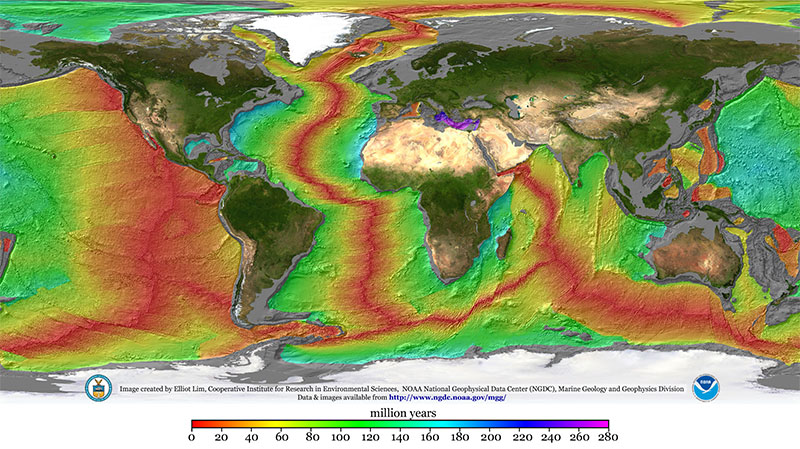
A map illustrating the age of the seafloor. Mid-ocean ridges stand out clearly in red. By sampling material from these ridges, planetary scientists can infer the composition of Earth’s deep interior. Click to enlarge. [Mr. Elliot Lim, CIRES and NOAA/NCEI]
That last option is especially exciting to present-day planetary scientists interested in constraining Earth’s formation history because it requires some very specific conditions. Since light noble gases like neon don’t dissolve well in seawater, they must have dissolved into a magma ocean — meaning the nebula was still around when Earth was large enough to have a molten surface. That already restricts us to a very specific time in the solar system’s history, but it doesn’t say much about the specific size of the proto-Earth other than “big,” and it doesn’t say much about the state of the nebula other than “it existed.” Recently, Vincent Savignac and Eve Lee (University of California, San Diego; McGill University) successfully refined these constraints to pin down information about both the early Earth and the nebula that surrounded it.
Infant Earths
Savignac and Lee began by growing a grid of infant Earths on their computers via models of gas accretion and atmosphere–magma interactions. Each simulation started with a different proto-Earth mass and nebular density, and each one yielded a different amount of neon in Earth’s deep interior. Excitingly, only a small handful of the scenarios tested ended up with values similar to those observed.
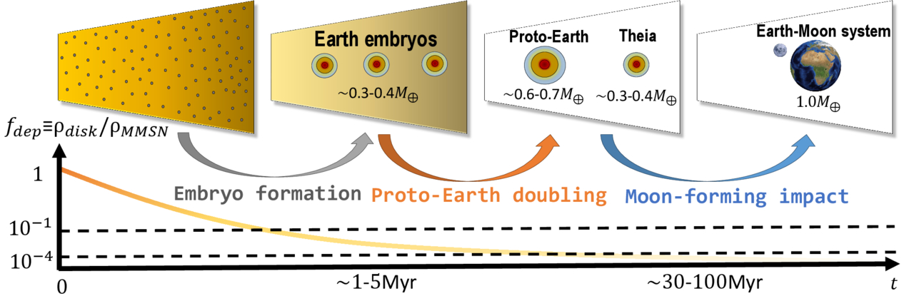
A schematic of Earth’s formation via embryo formation (when the noble gases enter the mantle) followed by mergers. Click to enlarge. [Savignac & Lee 2026]
Savignac and Lee demonstrated that these constraints are robust against the later stages of Earth’s evolution. In its later years, Earth either suffered or benefited from a giant impact, depending on your feelings about the Moon, but the researchers showed that this event doesn’t pose a problem for their models. Overall, this study builds a delightful link between rocks from our deep oceans and the particulars of Earth’s formation, demonstrating the unique power of planetary science to tie together different scientific fields.
Citation
“Constructing the Earth’s Formation History Using Deep Mantle Noble Gas Reservoirs,” Vincent Savignac and Eve J. Lee 2026 Planet Sci. J. 7 135. doi:10.3847/PSJ/ae64f7


![Plots showing stellar age and rotational velocity versus metallicity, [Fe/H].](https://aasnova.org/wp-content/uploads/2026/07/feltzingetal1-1.jpg)