")
Solving a Stellar Abundance Problem (with a Little Help from Our Oceans)
When solving mysteries about distant astronomical objects, sometimes it pays to take inspiration from sources closer to home. In today’s example, strange fluid behavior in the Earth’s oceans — combined with a healthy helping of magnetic fields — may provide the answer to a long-standing puzzle about the changing composition of red-giant stars.

Simulated salt fingers in fluids with decreasing Rayleigh numbers. The Rayleigh number determines whether heat in a system is transferred primarily through diffusion or convection. [Fariarehman; CC BY-SA 4.0]
A Possibility for Instability
Red giants undergo a process called dredge-up, during which their outer convective envelopes bring fusion products up to the surface, altering the chemical abundances there. After the dredge-up, surface abundances aren’t expected to change — yet observations show that they continue to evolve long after the dredge-up is complete. What drives this unexpected late-stage mixing in red giants?
One solution involves an instability called fingering convection. Fingering convection occurs in fluids with vertical gradients in temperature and chemical composition — a setup we see everywhere from the interiors of stars to Earth’s oceans. When the equilibrium of such a fluid is perturbed, the temperature diffuses more quickly than the chemical composition as the system seeks to reestablish equilibrium, triggering a runaway effect.
What does this look like in practice? Take the ocean as an example. The density of saltwater is determined by temperature and salt content, and warm saltwater often lies atop denser, colder water that is less salty. When a bubble of warmer water is pushed into the colder water beneath it, it cools quickly, but the salt is slow to diffuse outward. The cold, salty water is now denser than the water surrounding it, causing it to sink deeper. As this process continues, salt-rich “fingers” dive downward, eventually depositing the saltier water deep in the ocean.
The density of the material in stellar interiors depends on temperature, which diffuses rapidly, and chemical composition, which diffuses slowly — the perfect setup for fingering convection.
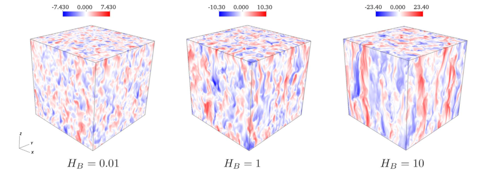
Vertical velocity of fluid parcels for three values of the Lorentz force coefficient, HB, which increases as the square of the magnetic field strength. Click to enlarge. [Harrington & Garaud 2019]
Chemical Mixing
Past modeling has shown that fingering convection does help mix chemical species in red-giant stars, but two orders of magnitude too slowly to explain observations. However, these simulations didn’t consider what effect magnetic fields — which are certainly present in the interiors of these stars — have on convection. What happens when we throw magnetic fields into the mix?
Peter Harrington and Pascale Garaud (University of California, Santa Cruz) used numerical models to explore the effect of magnetic fields on the rate of convection in stellar interiors. In their simulations, the authors apply a vertical background magnetic field of varying strength and randomly impose small perturbations in the temperature and composition. The perturbations grow as the instability takes hold, forming narrow fingers aligned with the magnetic field.
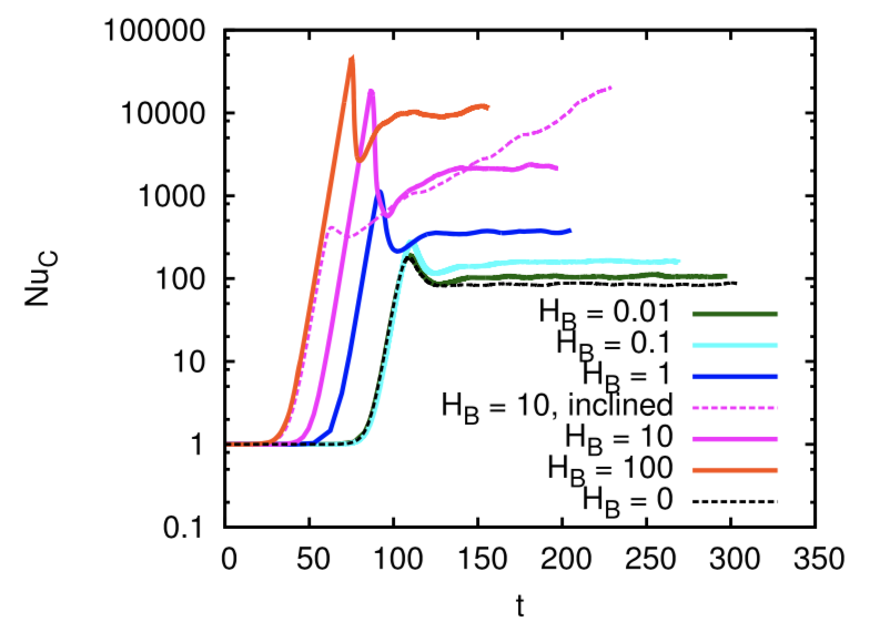
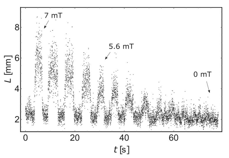
Evolution of the compositional Nusselt number (a measure of the strength of the vertical compositional transport) over time. Simulations with higher magnetic field strengths saturate more rapidly and reach higher rates of vertical transport. [Harrington & Garaud 2019]
Implications for Convection
The authors find that including magnetic fields in their simulations increases the rate of convection, with stronger magnetic fields leading to more rapid convection. For a purely vertical magnetic field of 0.03 Tesla (reasonable for stellar interiors), the convection rate increases by two orders of magnitude — enough to resolve the disagreement between theory and observations.
Magnetized fingering convection should affect more than just red giants; the authors note that main-sequence stars and white dwarfs should also exhibit this behavior, which needs to be accounted for when interpreting observed surface abundances.
Citation
“Enhanced Mixing in Magnetized Fingering Convection, and Implications for Red Giant Branch Stars,” Peter Z. Harrington & Pascale Garaud 2019 ApJL 870 L5. doi:10.3847/2041-8213/aaf812


