A Home for Another Fast Radio Burst
What causes fast radio bursts? Scientists are still hunting for the answer to this question — but the discovery of one burst’s nearby home may bring us a little closer to a solution.
Mysterious Pulses
More than a decade after their first discovery, fast radio bursts continue to pose a tantalizing mystery. These bizarre millisecond-duration pulses have been determined to be extragalactic in origin, yet we still don’t know what causes them. Could they be from merging black holes or neutron stars? Especially energetic supernovae? Collapsing pulsars? Or even something exotic, like cosmic string interactions?
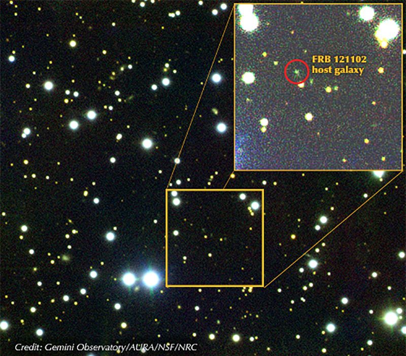
Visible-light image of the host galaxy of FRB 121102, previously the only fast radio burst that has been localized. [NRAO/ Gemini Observatory/AURA/NSF/NRC]
Typical or Unusual?
The only localized burst, FRB 121102, resides in a bright, star-forming region in the outskirts of a low-metallicity dwarf galaxy. But FRB 121102 is unusual among fast radio bursts: it’s the only burst observed to repeat, and its environment appears to be more highly magnetized than those of other bursts.
Is FRB 121102 is representative of the general population of fast radio bursts, or do its unique characteristics mean that it’s caused by something completely different than the rest of the population? Our best bet for answering this question is to find the homes of more bursts — and now we may be in luck.
A Plausible Home Found
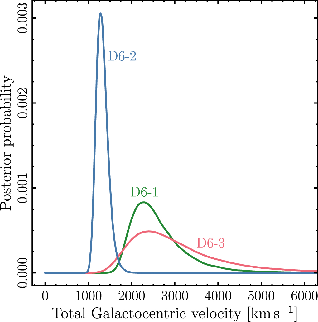
Led by Elizabeth Mahony (CSIRO Astronomy and Space Science, Australia), a team of scientists has discovered the likely home of a recent fast radio burst, FRB 171020. This burst’s dispersion measure — a measure of the amount of matter the signal traveled through to get to us — is the lowest of all known fast radio bursts, indicating that this burst originated relatively close to us.
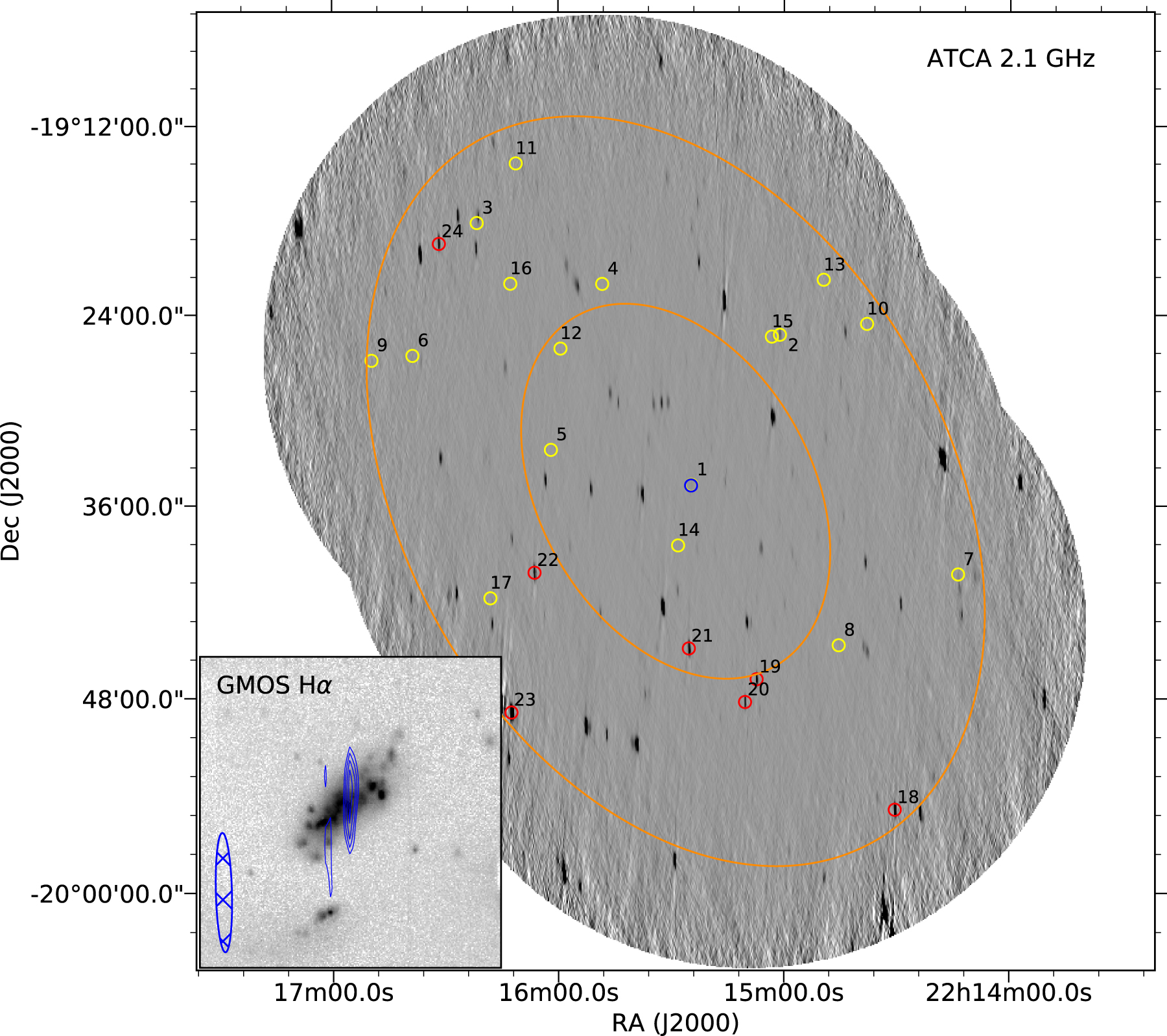
Australia Telescope Compact Array (ATCA) radio continuum image indicating the localization region of FRB 171020. Small circles mark candidate host galaxies for the burst. The blue circle marks the most likely candidate, ESO 601–G036. The inset shows a zoomed-in view of this galaxy. [Mahony et al. 2018]
Missing Persistence
Intriguingly, ESO 601–G036 is both similar to and different from the host galaxy of FRB 121102. The two galaxies are alike in size, they have similarly low metallicities, and they have similar star formation rates.
But FRB 121102’s host galaxy harbors a persistent compact radio source — a source that continuously emits bright radio emission. Some astronomers have even proposed that detecting such persistent radio emission may be a way to identify fast-radio-burst hosts in the future. In contrast, ESO 601–G036 shows no sign of a persistent radio source — nor does any other galaxy in the volume of space from which FRB 171020 could have originated.
The nearness of the potential home found for FRB 171020 will provide us with a convenient opportunity to learn about this host environment in more detail in the future. Meanwhile, the contrast of this galaxy to the host galaxy of FRB 121102 seems to support the idea that there may be different types of fast radio bursts with different origins.
Citation
“A Search for the Host Galaxy of FRB 171020,” Elizabeth K. Mahony et al 2018 ApJL 867 L10. doi:10.3847/2041-8213/aae7cb