A Black Hole X-Ray Binary Rises
New observations have captured a feeding black hole in our galaxy as it bursts onto the scene.
Bursting Binaries
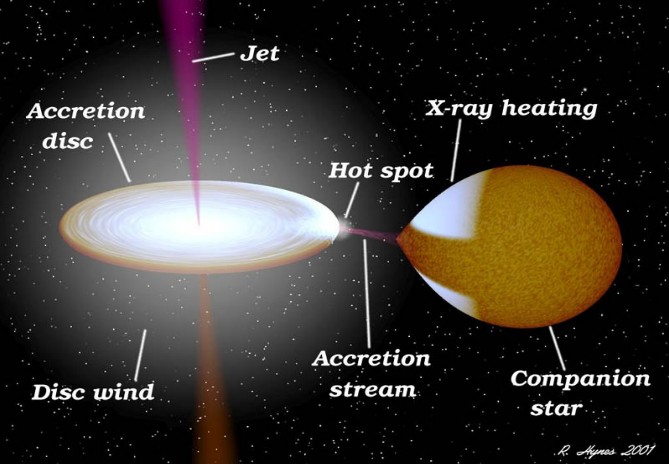
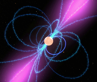
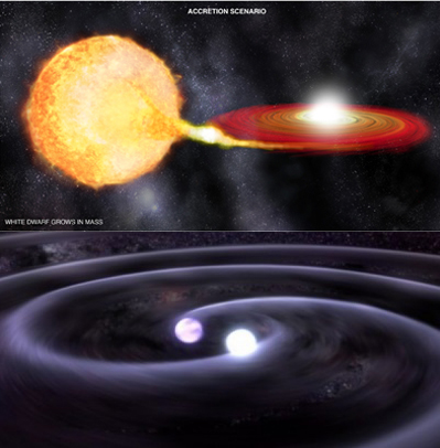
This representation of an X-ray binary shows the accretion disk that surrounds the black hole. According to models, instabilities in this accretion disk can lead to the binary going into outburst. [NASA/R. Hynes]
X-ray binaries come in two main types, depending on the size of the donor star: low-mass and high-mass. In a low-mass X-ray binary (LMXB), the donor star typically weighs less than one solar mass. One type of LMXB, known as a transient/outbursting LMXB, has a peculiar quirk: though they often go undetected in their dim, quiescent accretion state, these sources exhibit sudden outbursts in which the brightness of the system increases by several orders of magnitude in less than a month.
Where do theses outbursts begin? What causes the sudden eruption? What else can we learn about these odd sources? Though theorists have built detailed models of transient LMXBs, we need observations that can confirm our understanding. In particular, most observations only capture transient LMXBs after they’ve transitioned into an outbursting state. But a sneaky telescope has now caught one source in the process of waking up.
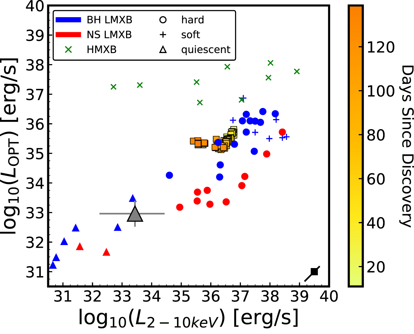
ASASSN-18ey’s position on an X-ray vs. optical luminosity diagram, shown with orange and yellow markers as it evolves through its outburst, place it within the region dominated by black hole LMXBs (blue markers) throughout the outburst. [Tucker et al. 2018]
Sudden Discovery
The All-Sky Automated Survey for SuperNovae (ASAS-SN, pronounced “assassin”) regularly scans the sky hunting for transient sources. In March of this year, it spotted a new object: ASASSN-18ey, a system roughly 10,000 light-years away that shows all the signs of being a new black-hole LMXB.
ASASSN-18ey’s initial discovery prompted a flurry of follow-up observations by astronomers around the world. As of 1 October 2018, the tally had hit more than 360,000 observations — giving ASASSN-18ey the potential to be the best-studied black-hole LMXB outburst to date.
In a recent publication led by Michael Tucker (Institute for Astronomy, University of Hawai’i), a team of scientists details what we know about ASASSN-18ey so far, and what it can tell us about how LMXBs behave.
Confirming Models
What makes ASASSN-18ey unique is its discovery in optical wavelengths before X-ray. Tucker and collaborators use the various observations of this source to determine that there was a ~7.2-day lag between the flux rises in the optical and the X-ray light curves.
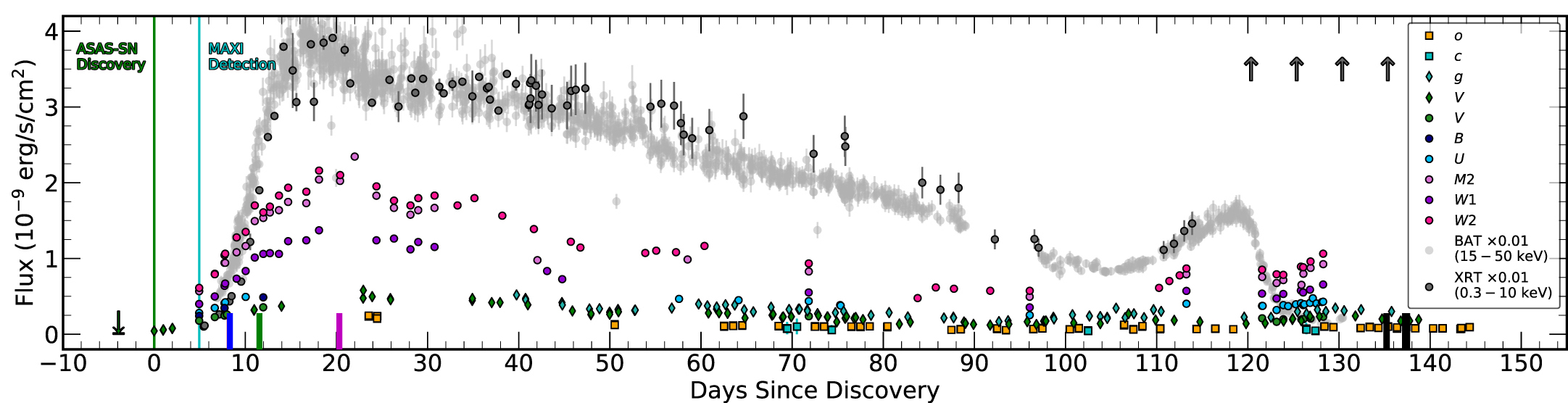
The full light curves of ASASSN-18ey from ASAS-SN, ATLAS, and Swift show the source’s rapid rise to outburst state. Click to enlarge. [Adapted from Tucker et al. 2018]
Further observations of ASASSN-18ey as it continues to evolve will undoubtedly shed more light on the state transitions and behavior of LMXBs. In the meantime, we can enjoy this sneaky look at a new black hole LMXB system on the rise.
Citation
“ASASSN-18ey: The Rise of a New Black Hole X-Ray Binary,” M. A. Tucker et al 2018 ApJL 867 L9. doi:10.3847/2041-8213/aae88a