
A Vampire’s Sandwich Filled with Gas and Dust
Editor’s Note: Astrobites is a graduate-student-run organization that digests astrophysical literature for undergraduate students. As part of the partnership between the AAS and astrobites, we occasionally repost astrobites content here at AAS Nova. We hope you enjoy this post from astrobites; the original can be viewed at astrobites.org.
Title: Dracula’s Chivito: Discovery of a Large Edge-On Protoplanetary Disk with Pan-STARRS
Authors: Ciprian T. Berghea et al.
First Author’s Institution: US Naval Observatory
Status: Published in ApJL
Where Planets Are Born
Studying protoplanetary disks helps us understand how planets, including those in our solar system, are born. These disks are vast and flared structures, consisting of dust and gas orbiting a young star. Protoplanetary disks contain the remnants of the stellar birth process, in which a collapsing molecular cloud gives rise to a central star surrounded by a swirling disk of material. Protoplanetary disks are vital to observe as they are the birth sites of planets. The tiny dust particles come together, sticking to each other and forming larger bodies. This process, influenced by gravity, gas, and radiation, leads to the birth of planets in developing planetary systems.
Meet the Vampire Sub
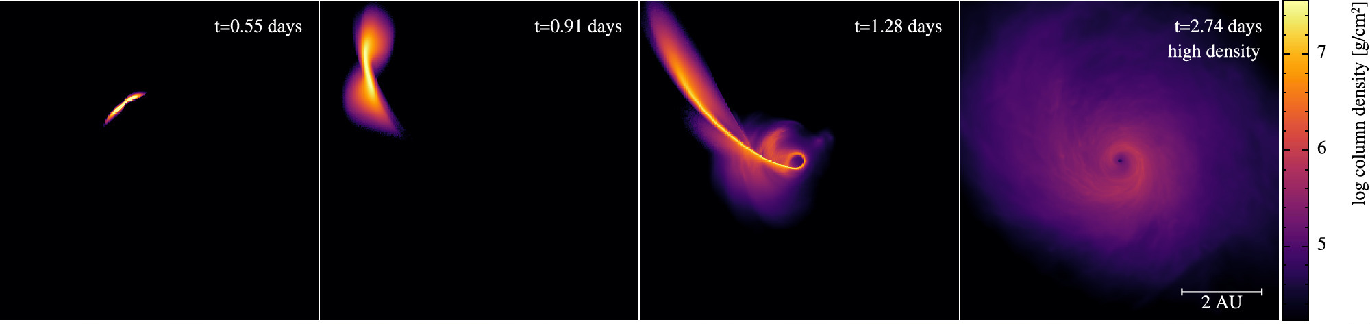
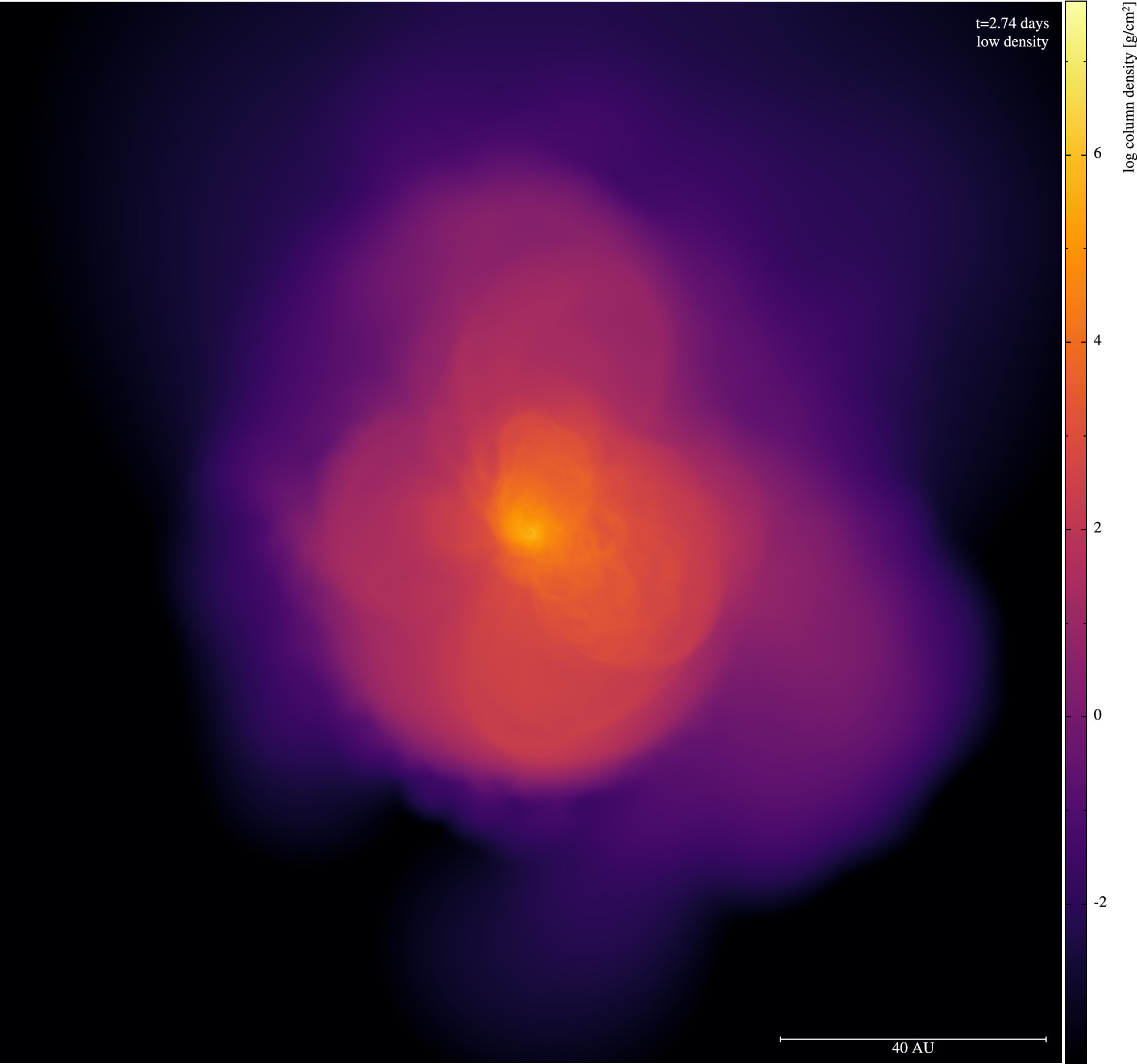
This research article features a large edge-on protoplanetary disk that was stumbled upon when going through images from the Pan-STARRS research project as a part of a study of active galactic nucleus candidates. This disk is one of the largest known disks in the sky and is oriented edge on, completely obscuring its central star. Associated with a source of infrared light in the same region of the sky, IRAS 23077+6707, the disk spans approximately 11″ in apparent size, with a very faint structure in the disk’s northern part extending out to about 17″. It is possibly the largest protoplanetary disk (by angular extent) discovered to date. The structure of this disk is reminiscent of the popular Gomez’s Hamburger, which is not associated with any star-forming region, just like the subject of this article. The similarity to a sandwich, along with the fang-like structures in the northern part of the disk as seen in the images in Figure 1, earned the IRAS 23077+6707 protoplanetary disk the name “Dracula’s Chivito” (chivito is a type of sandwich and the national dish of Uruguay, where one of the co-authors is from).

Figure 1: Pan-STARRS image of Dracula’s Chivito (left) and the associated radiative transfer model (right). In the northern part of the disk, very faint filaments are seen extending 17″ out from the edges of the disk. These filaments have been nicknamed “fangs.” These are interpreted as the edges of the disk envelope, as reproduced in the model image. These fangs are likely obscured by a cloud in the southern part of the disk. [Adapted from Berghea et al. 2024]
Decoding DraChi
Analysis: Images of Dracula’s Chivito (henceforth referred to as DraChi) were obtained in the grizy filters of Pan-STARRS (Figure 1). These images and data from the Galaxy Evolution Explorer (GALEX) (ultraviolet), the Two Micron All-Sky Survey (2MASS) (infrared), the Infrared Astronomical Satellite (IRAS) (infrared), and AKARI (infrared) were used for photometric analysis, i.e., flux or brightness measurements. These data were used to construct the spectral energy distribution of the disk (Figure 2), together with a radiative transfer model generated using the code HOCHUNK3D. Radiative transfer models help us understand the disk geometry and how light is scattered by the dust grains in the disk. This light, which we see along our line of sight, is plotted as a spectral energy distribution. Spectral energy distributions give information about how much energy an object gives off at different wavelengths.
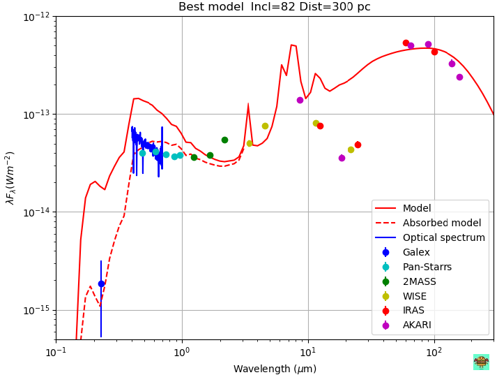
Figure 2: The spectral energy distribution of the disk, using photometric data from the image, the model, and other sources as mentioned in the article. Brightness is plotted as a function of wavelength. The data (colored dots) match the model (the solid red line shows the model without extinction, and the dashed red line shows the model with extinction) in most places except in near- and mid-infrared wavelengths, which could be due to discrepancies between instruments or possible variability in the disk’s luminosity. [Berghea et al. 2024]
Basic Properties: The spectral energy distribution suggests that the host star of the disk is a pre-main-sequence star of type A with a temperature of about 6500–8500K. The images of the disk and the resultant radiative transfer model constrain the disk inclination to be between 80° and 84°. The scale height of the disk is about 25–50 au at a radius of 500 au (astronomical units), where 1 au is the distance from Earth to the Sun. Using the distance and the angular extent of the disk in the sky, the disk’s radius is estimated to be 1,650 au. The radiative transfer model, based on the scattering of the light, quantifies the mass of the disk to be about 0.2 times that of the Sun.
The Fangs: The authors noticed two “fang-like” features in the northern part of the disk, and these features were also reproduced in the model of the disk. The “fangs” closely resemble the “edge” of the shadow created by the disk in the bright surrounding envelope. They could be filaments due to a possible outflow from the central part of the disk, which is characteristic of a young disk at the end of the Class I phase (~0.5 million years old). It is possible that the fangs are present in the south, but this region is likely obscured in the images from Pan-STARRS and could be perhaps seen in infrared (longer-wavelength) imaging.
Is DraChi the Only One?
The short answer is no. DraChi is certainly different from most other protoplanetary disks, given its size and large distance from any known star-forming regions. But the existence of Gomez’s Hamburger proves there are more such disks awaiting discovery. A disk as young as DraChi is vital to understanding planet formation in its earlier stages, and its large size makes for interesting future observations using more sensitive instruments.
Original astrobite edited by Kylee Carden and Jessie Thwaites.
About the author, Maria Vincent:
Maria is a PhD candidate in astronomy at the Institute for Astronomy, University of Hawai’i at Manoa. Her research focuses on adaptive optics and high-contrast imaging science and instrumentation with ground-based telescopes. Driven by a fascination with planet formation and the intricate processes shaping our solar system, she uses the Subaru Coronagraphic Extreme Adaptive Optics suite to observe and study morphological features of protoplanetary disks in near-infrared wavelengths, aiming to understand disk structure and processes governing planet formation. On the instrumentation side, she is working on designing and constructing an optical testbed to test and characterize a new deformable mirror as part of the upcoming High-order Advanced Keck Adaptive Optics upgrade. Outside of work, she enjoys blogging, mystery, historical and science fiction literature and cinemedia, photography, hiking, and travel.


 Hunting in Gamma-ray Bursts")


