Editor’s note: Astrobites is a graduate-student-run organization that digests astrophysical literature for undergraduate students. As part of the partnership between the AAS and astrobites, we occasionally repost astrobites content here at AAS Nova. We hope you enjoy this post from astrobites; the original can be viewed at astrobites.org!
Title: Possible Photometric Signatures of Moderately Advanced Civilizations: The Clarke Exobelt
Author: Hector Socas-Navarro
First Author’s Institution: University of La Laguna, Spain
Status: Accepted to ApJ
The Search for Extraterrestrial Intelligence
The detection of extraterrestrial intelligence is a quest that has fascinated astronomers since we first realized that there were worlds beyond our own.
Listening projects, like SETI@home and Breakthrough Listen, look for possible signals from other civilizations. Such a discovery would unequivocally prove that we are not alone. However, in order to efficiently transmit a message across interstellar space, a civilization would likely beam it as tightly as possible towards its destination. That means that we wouldn’t be able to eavesdrop if we weren’t in line with the beam.
Another possible detection method is analyzing an exoplanet’s atmosphere with spectroscopy. As a planet passes in front of its star, a portion of the light from that star will be absorbed by the planet’s atmosphere. Analyzing the way the observed spectrum changes as the planet transits can tell us the planet’s atmospheric composition. A similar method may be applied by using light reflected off the planet’s atmosphere. Once we know what molecules are present in the planet’s atmosphere, we could search for chemical signs of life. Certain species of gas, like oxygen, could be the result of life on the planet’s surface. Some, such as chlorofluorocarbons (CFCs), would be highly indicative of the presence of an industrial civilization. While such a discovery would not be a direct detection of alien life, it would provide strong evidence for its presence.
A New Detection Strategy
In this paper, Socas-Navarro presents a new potential way to detect moderately advanced civilizations. A civilization that has reached or surpassed our own level of technology may have a great number of satellites in orbit around its planet. In particular, a good place to look for these satellites is in geosynchronous orbit. In geosynchronous orbit, a satellite has an orbital period that matches the rotation period of the planet. Thus, it remains directly over one spot on the planet. These orbits are useful because they allow a satellite to maintain contact with its base station at all times. For example, many of the Earth’s communications and navigations satellites are in geosynchronous orbit. If other civilizations use satellites for similar purposes, they would likely also make use of geosynchronous orbits.
In order to remain in geosynchronous orbit, a satellite must stay at a particular distance from its planet. If it comes closer, it will orbit faster than the Earth rotates, and if it is too far away, it will go slower than the Earth rotates. However, these orbits can have some slight inclinations. If the orbit is inclined, the satellite will not remain directly overhead, but will trace out a small analemma over a sidereal day. The author coins the term “Clarke exobelt” (CEB) to describe the satellites in this region of space around a planet.
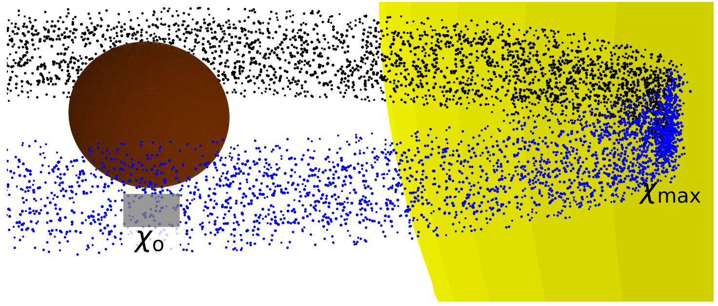
Figure 1: An illustration of the Clarke exobelt. Each small dot represents a satellite in geosynchronous orbit around the planet, the brown sphere. The yellow sphere on the edge represents the star. Here, the size and density of satellites have been greatly exaggerated. The opacity, χ, increases from the face (χo) towards the edge (χmax). [Socas-Navarro 2018]
As can be seen in Figure 1, a high density of satellites in geosynchronous orbit will create a thick band which could block out light from the star. The more satellites, the more light they will block. This opacity will block more light from the star than the planet alone, resulting in a noticeable difference in the transiting planet’s light curve. An example of what a light curve affected by Earth’s CEB might look like is shown in Figure 2. As the planet moves between us and its star, the light we receive from the star will decrease. If the planet does not have a CEB, the light curve will exhibit a relatively flat decline. However, if there is a thick band of satellites around it, these will begin to obscure the light from the star before the planet is fully in front. This will result in a small dip right before the main transit happens. It will also cause more light to be blocked overall, resulting in a deeper light curve.
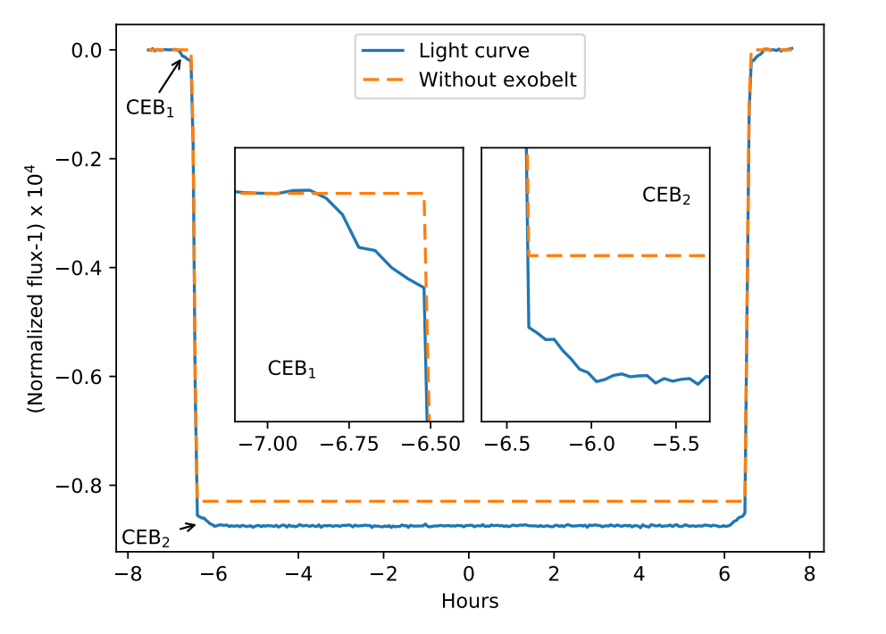
Figure 2: An example light curve for an Earth-like planet transiting a Sun-like star. The orange dashed line represents what the light curve will look like during a transit if there is no CEB. The blue line is a simulation of what the light curve would look like with a large number of satellites in geosynchronous orbit. Note how the light curve with the CEB is deeper, and the corners are rounded at the beginning and end of the transit. [Socas-Navarro 2018]
Based on publicly available databases, the author identifies 1,738 satellites in geosynchronous orbit around the Earth. This is a low estimate, because these databases do not include decommissioned satellites, space junk, or classified satellites. For the past 15 years, the number of satellites in geosynchronous orbit has been increasing exponentially. The author predicts that at this rate, within 200 years, our CEB will be thick enough that it could be observed from nearby stars by civilizations with the same detection capabilities as us.
The author puts forth several other simulated light curves for systems of interest, including TRAPPIST-1. In each case, the simulations use the telescope specifications of the Kepler mission, making these possible to be detected using our own technology.
In order to determine if the shape of a light curve is from a CEB, and not caused by some other effect, it is important to know how far from the planet the CEB would be. This would allow researchers to model what the light curve should look like with and without a CEB.
The orbital radius (rC) of the CEB depends on the mass (M) and rotational period (T) of the planet as rC3 = (GMT2)/(4π2}. An estimation of the planet’s mass can be made by using the transit photometry to find its size. Assuming the planet has a density similar to the Earth, we can calculate its mass. The rotational period, on the other hand, is more difficult to find. Future observations may be able to create surface maps of planets to determine rotational periods. While this has not yet been done, studies show that this could be possible for planets up to 5 parsecs away. If the planet is tidally locked to its star, the rotation would be straightforward to find. Tidal locking may be very common for planets orbiting in their star’s habitable zone, making it possible for astronomers to at least approximate the planet’s rotational period.
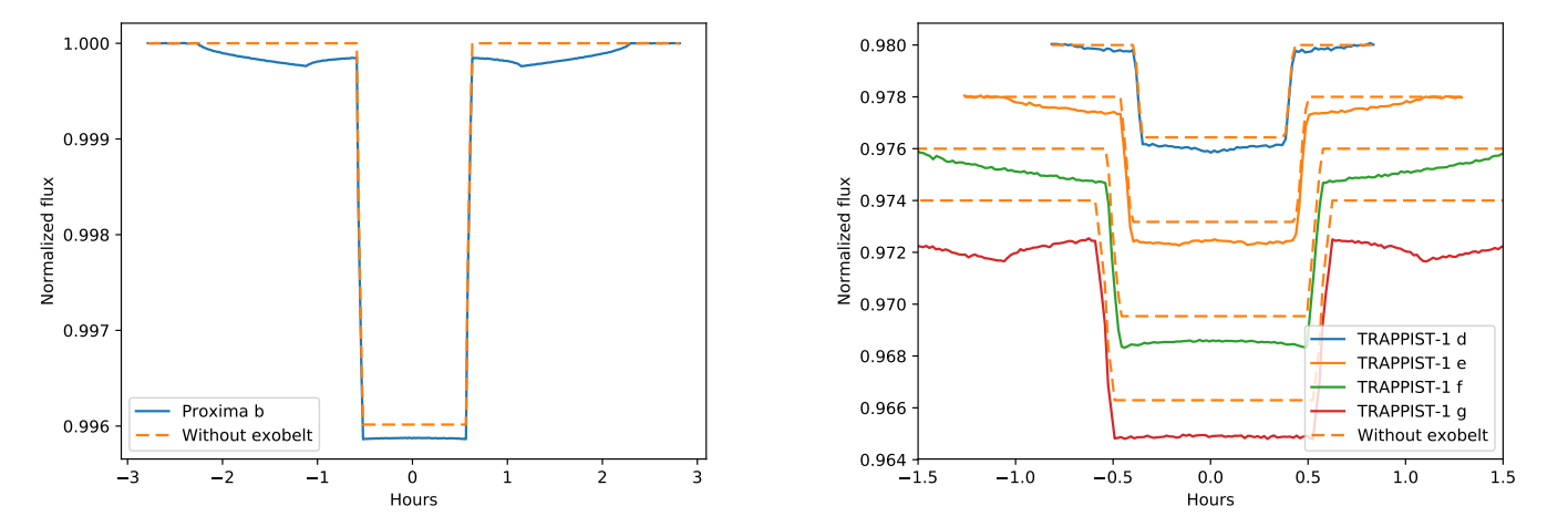
Figure 3: Light curves for the Proxima b and TRAPPIST-1 systems. Like in Figure 2, these show the light curve of a planetary transit without a CEB (dashed line) and with one (solid line). [Socas-Navarro 2018]
Finally, the author examines whether or not such a light curve could occur naturally. A planetary ring system could produce a similar light curve pattern. However, as the author points out, evidence from our own Solar System suggests that rings only form outside of the frost line. This is beyond the star’s habitable zone, making it unlikely that life like ours would develop out there. There is also no reason a ring system would prefer to form in geosynchronous orbit instead of any other inclination. While this orbital band is of high use to a civilization, there is no natural preference for it. Ring systems also tend to be very flat. Objects in the rings are spread out over the radial direction, but do not have much thickness in inclination. Geosynchronous orbits, on the other hand, are very thin radially, but have a thicker inclination. This will create a slightly different signal, which could be detected.
Are They Out There?
Many of the ideas presented in this paper are still speculation. These are extrapolations of what we know about civilization here on Earth. Aliens might not use geosynchronous orbits enough to create a thick band of satellites. They may be significantly more advanced than us, and have no need for a large number of satellites. Or they could be much less advanced than us, without the capability to get into orbit. The nearest civilization to us might even be too far away for us to be able to see its CEB. When discussing alien civilizations, it is important to keep in mind that we have very little data to base our ideas on, and we must make many assumptions.
Speculative though it may be, the method presented in this paper is another tool in our kit we can use on our search for extraterrestrial intelligence. This technique represents a way we can search for alien civilizations with our current detection capabilities. It relies only on technologies that we know are possible. Upcoming missions like the James Webb Space Telescope and TESS could apply this method to search for an alien civilization.
About the author, Peter Sinclair:
I’m a graduate student at the University of New Mexico. My hobbies include reading, cooking, and playing board and video games. You can find me on Twitter @Phiteros and on my blog, themodernpolymath.com.


