
A White Dwarf Moving With The Flow
Editor’s note: Astrobites is a graduate-student-run organization that digests astrophysical literature for undergraduate students. As part of the partnership between the AAS and astrobites, we occasionally repost astrobites content here at AAS Nova. We hope you enjoy this post from astrobites; the original can be viewed at astrobites.org!
Title: A Young Ultramassive White Dwarf in the AB Doradus Moving Group
Author: Jonathan Gagné, Gilles Fontaine, Amélie Simon, & Jacqueline K. Faherty
First Author’s Institution: Carnegie Institution of Washington DTM
Status: Published in ApJL
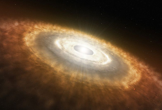
Figure 1: Artist’s impression of a white dwarf. [All About Space/Imagine Publishing]
A co-moving group of stars is just what it says on the tin: a group of stars that are all moving in about the same direction at about the same speed. Such a group is normally around a couple of dozen stars. They’re generally not too far away from each other in space as well, but they’re not nearly as tightly bunched up as clusters are; the space inside a co-moving group can contain many stars that aren’t part of the group. For instance, the Ursa Major moving group includes most of the brightest stars in the Big Dipper, and it also extends to include some stars at the far end of the sky in Triangulum Australe, but it does not include the Sun — even though the Sun is between the two. Stars in a co-moving group are generally thought to have formed all at once, perhaps as part of an open cluster that has broken apart. This shared history can make co-moving groups useful for constraining models of stellar evolution.
One of the closest co-moving groups is the AB Doradus moving group, a group of about 30 stars centred about 20 parsecs away from the Earth. A possible member of the group for some time has been a white dwarf called GD 50, but there have never been precise enough data on the star to know for sure. If true, GD 50 would be the only white dwarf in the group. This makes it interesting for stellar evolution purposes, as it would provide a new window onto the stellar history of the group. White dwarf models have their own set of strengths and weaknesses that differ from those for main sequence stars; for instance, the age of a white dwarf can generally be determined much more precisely than a main sequence star.
Testing Membership
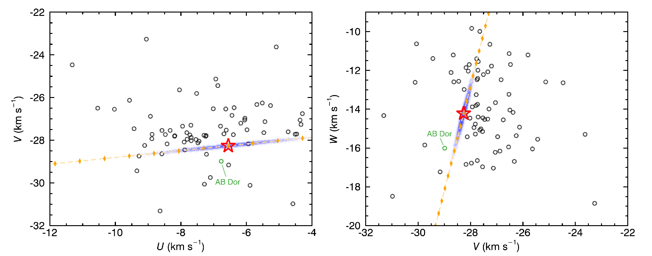
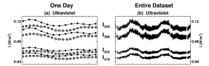
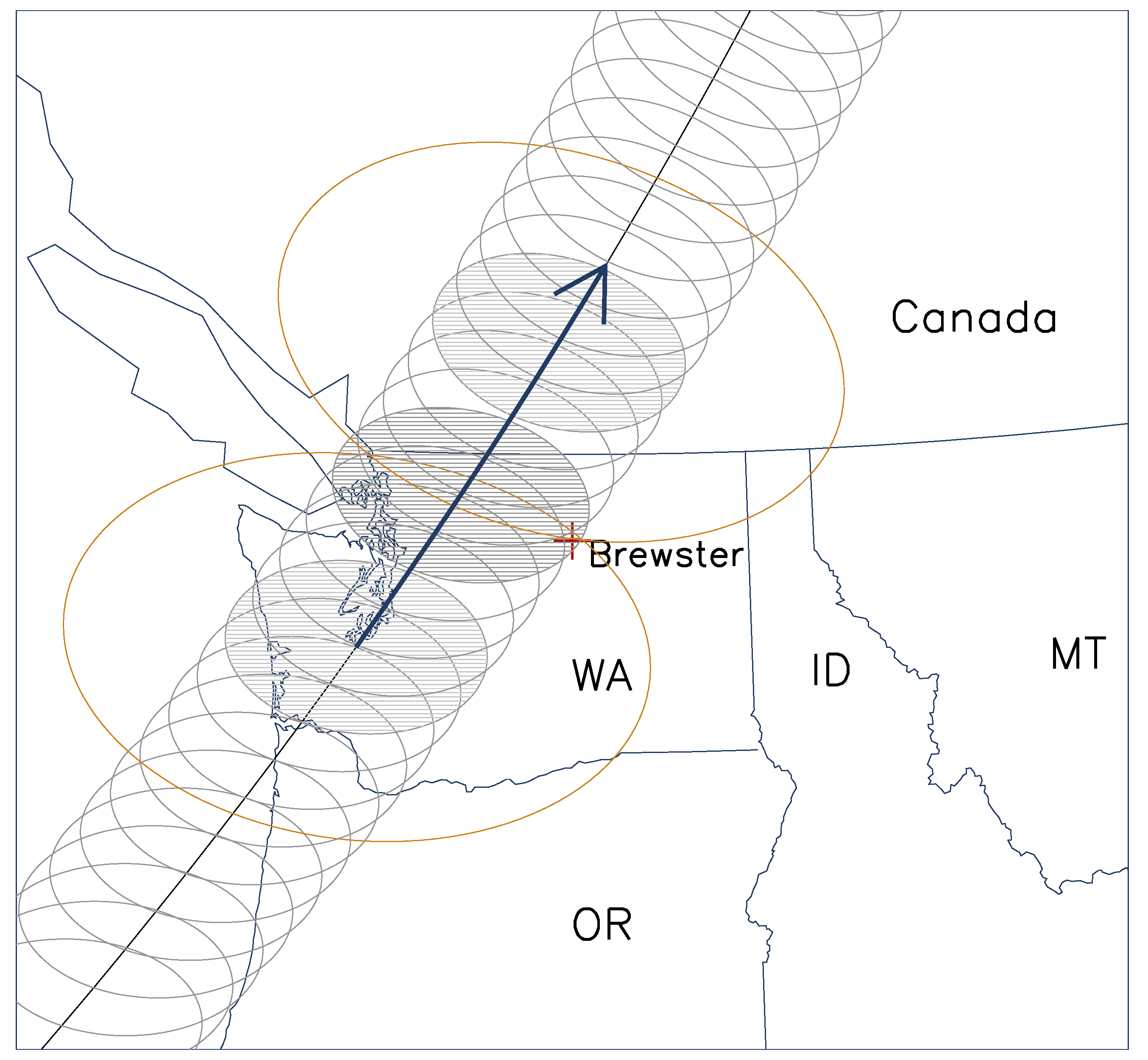
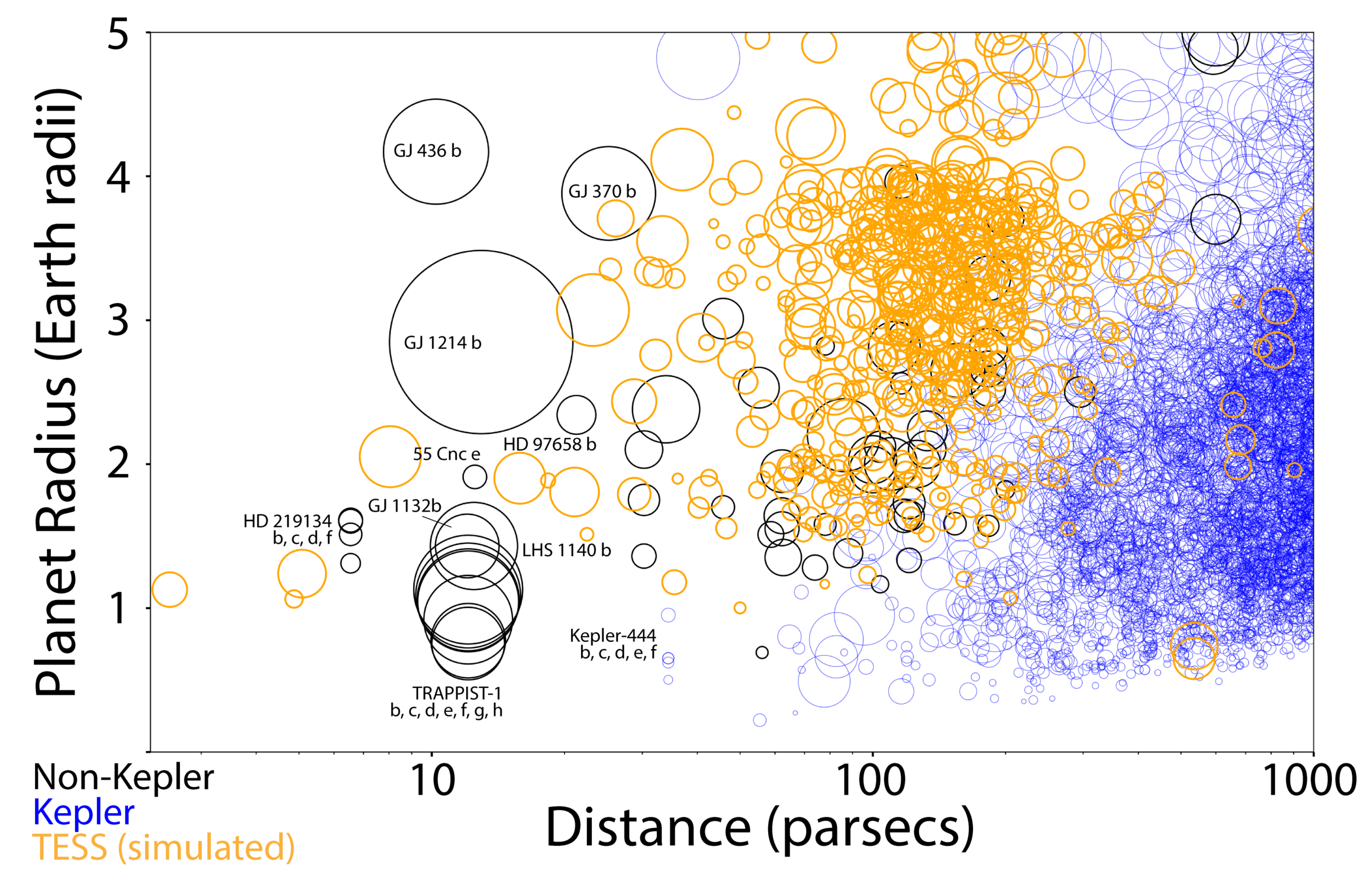
Figure 2: The measured velocity of GD 50 (shown as a red star) compared with other members of the AB Dor group of stars. U, V and W refer to velocity components in each of three different directions (see text). Because the spectroscopic radial velocity of GD50 is much less certain than other velocity measurements, the yellow dashed line here shows the direction in which GD 50 would move if its radial velocity were to change, and the spread of purple dots show randomly-generated models spread around the best-fit value to give an idea of the uncertainty. The star called AB Dor, after which the co-moving group is named, is highlighted in green. [Gagné et al. 2018]
, as well as measuring the proper motions (motion across the sky) of those stars. By combining these with a spectroscopic measurement of the star’s velocity towards or away from the Earth, we can pin the star down quite well in both position and velocity space.
In order to test whether GD 50 really belongs to the AB Dor group, the authors took the position and velocity of the star in three dimensions (away from the Galactic centre, around the Galactic centre, and up-and-down relative to the Galactic plane) to give six properties. For each property, they modelled the group as having a Gaussian distribution, and they found the probability of a group member having the property measured for GD 50. They compared this to the probability of the star being just any old member of the galactic field by modelling the local galactic field as a more complex combination of 10 Gaussians. Overall, they found a 99.7% likelihood that the star is a part of the AB Dor group (see Fig 2).
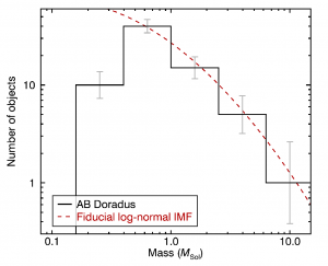
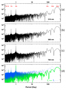
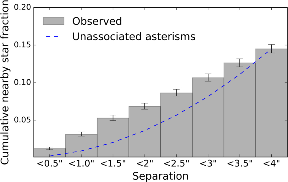
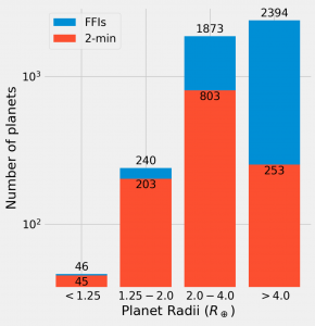
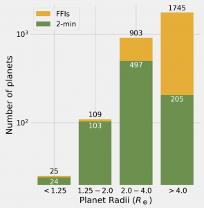
Figure 3: Histogram of initial stellar masses in the AB Dor group. The right-most bin includes only one object, which is the main sequence star that evolved into GD 50. The red dashed line shows a model distribution for inital stellar masses. For the 4 highest-mass bins the model agrees well. The lowest-mass bin has fewer stars than the model predicts. This is probably due to the selection effect against low-mass, faint stars — ie, these stars exist but we haven’t detected them yet. Source: Figure 3 in today’s paper.
The History of GD 50
So what do we know about GD 50, and what can this tell us about the AB Dor group? Firstly, we know what kind of main sequence star GD 50 evolved from. Stars lose most of their mass as they evolve into white dwarfs, but this process is pretty well understood. GD 50 is a pretty heavy white dwarf, with a mass 1.28 times the mass of the Sun. This means that, as a main-sequence star, it must have come in at about 7.8 times the mass of the Sun. This would make it the only star in the AB Dor group with this much mass, but given models of initial mass functions for clusters, we would expect the group to contain around one star this massive (see Fig 3).
We can also tell the age of GD 50 quite well based on models of stellar evolution and white-dwarf cooling — the first tells you how long a star of 7.8 solar masses would live, and the second tells you how long it must have been a white dwarf in order to match GD 50’s temperature. Today’s authors find a total age for GD 50 of 117 +/- 22 million years. Previous estimates for the age of the AB Dor group gave around 130-200 million years, so the estimate in today’s paper is a touch shorter and quite a lot more tightly constrained. This puts the AB Dor group among the youngest known nearby co-moving groups.
Overall, the identification of GD 50 as part of the AB Dor group allows us to put some constraints on the history of that group, and gives us a way to check previous measurements of properties like the group’s age. The data from Gaia is only beginning to make its impact, and we can hope that, in the future, more results like this will be found and help us to build towards a better understanding of the histories of these stellar groups.
About the author, Matthew Green:
I am a PhD student at the University of Warwick. I work with white dwarf binary systems, and in particular with AM CVn-type binaries. In my spare time I enjoy writing of all kinds, as well as playing music, board games and rock climbing. For more things written by me, take a look at my website.


 ), some nitrogen atoms are converted to carbon atoms following this process:
  .
.

