 Binary Neutron Star Merger Simulations")
59 (Fifty-Nine!) Binary Neutron Star Merger Simulations
Editor’s note: Astrobites is a graduate-student-run organization that digests astrophysical literature for undergraduate students. As part of the partnership between the AAS and astrobites, we occasionally repost astrobites content here at AAS Nova. We hope you enjoy this post from astrobites; the original can be viewed at astrobites.org.
Title: Binary Neutron Star Mergers: Mass Ejection, Electromagnetic Counterparts and Nucleosynthesis
Authors: David Radice, Albino Perego, Kenta Hotokezaka, Steven A. Fromm, Sebastiano Bernuzzi, Luke F. Roberts
First Author’s Institution: Princeton University
Status:Submitted to ApJ
Neutron star mergers are absolutely fascinating. These events are not just sources of gravitational waves but of electromagnetic radiation all across the spectrum — and of neutrinos as well. If you missed the amazing multimessenger observations last year that gave us a peek into what binary neutron star (BNS) systems are up to, please check out this bite about GW170817! The observations had major implications for many fundamental questions in astrophysics. The gravitational-wave signal from the merger was detected along with the electromagnetic radiation produced. As a result, we were able to confirm that neutron-star mergers are sites where heavy elements (those beyond iron) can be made via the r-process.
While all of this has undoubtedly been extremely cool (and we’re holding our collective breath for more data), there’s a lot of work that remains to be done. We need accurate predictions of the quantity and composition of material ejected in mergers in order to fully understand the origin of the heavy elements, and to say whether BNS mergers are the only r-process site. To investigate such questions, we require theoretical models that include all the relevant physics. Today’s paper presents the largest set of NS merger simulations with realistic microphysics to date. By realistic microphysics, we mean that the simulations also take into account what the atoms and subatomic particles are doing. This is done by using nuclear-theory-based descriptions of the matter in neutron stars, and by including composition and energy changes due to neutrinos (albeit in an approximate way).
Simulating Neutron-Star Mergers
Modeling BNS mergers is a complex multi-dimensional problem. We need to simulate the dynamics in full general relativity, along with the appropriate microphysics, magnetic fields and neutrino treatment. Remarkable progress has been made, particularly in the last decade, since the first purely hydrodynamical merger simulations were carried out. Still, the problem remains extremely computationally expensive and simulation efforts have traditionally focused either on carrying out general relativistic simulations while sacrificing microphysics, or on incorporating advanced microphysics with approximate treatments of gravity. If you care about the merger dynamics and the dynamical ejecta, i.e., material ejected close to the time of merger due to tidal interaction and shocks, you need fully general relativistic simulations, like the ones presented in today’s paper.
The authors carry out 59 high-resolution numerical relativity simulations, using binaries with different total masses and mass ratios. They also use different descriptions of the high-density matter in neutron stars. Neutrino losses are included in all cases, and some simulations include neutrino reabsorption as well. A few simulations even include viscosity. The authors systematically study the mass ejection, associated electromagnetic signals, and the nucleosynthesis from BNS mergers.
Mass Ejection

Fig 1. Electron fraction for an example simulation. The neutron stars are 1.35 Msun each and neutrino reabsorption has been included. The bulk of the ejecta lies within a ~60 degree angle of the orbital plane. [Radice et al. 2018]
The authors also find a new outflow mechanism, aided by viscosity, that operates in unequal mass binaries. This ejecta component, called “viscous-dynamical ejecta”, is discussed in detail in a companion paper.
Using their results, the authors fit empirical formulas that predict the mass and velocity of ejecta from BNS mergers. Even more material can become unbound from the remnant object on longer timescales (“secular ejecta”), but this is not studied here due to the high computational costs of running the simulation for that long.
Nucleosynthesis
The authors study in detail how the r-process nucleosynthesis depends on the binary properties and neutrino treatment. Sample nucleosynthesis yields are presented in Fig 2. You’ll notice that the second and third r-process peaks are robustly produced while the first peak shows more variation. In fact, the first peak is quite sensitive to the neutrino treatment as well as the binary mass ratio.
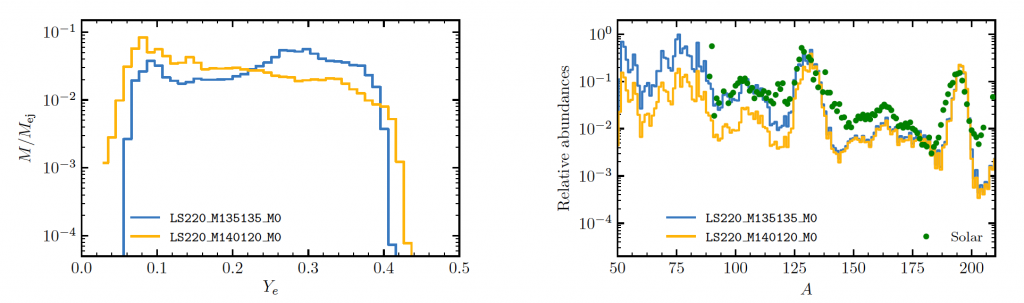
Fig 2. Electron fraction (left) and nucleosynthesis yields (right) of the dynamical ejecta. “A” refers to the mass number of the nucleus. The different colored lines represent binaries with different mass ratios. The green dots show solar abundances. [Radice et al. 2018]
Electromagnetic Signatures
The radioactive decay of the r-process nuclei produced powers electromagnetic emission, referred to as a “kilonova”. Other electromagnetic signals can also be produced due to different ejecta components.
The authors compute kilonova curves for all their models. They find that binaries that form black holes immediately after merger do not have massive accretion disks and produce faint and fast kilonovae. When the remnants are long-lived neutron stars, more massive disks are formed and the kilonovae are brighter and evolve on longer timescales. Example kilonova curves are shown in Fig 3.
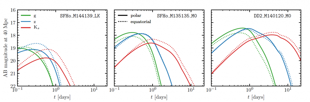
Fig 3. Kilonova curves in three bands for three different models: binary with prompt BH formation (left), binary forming a hypermassive neutron star (middle), binary forming a long-lived supramassive NS (right). Solid and dashed lines correspond to the viewing angle. [Radice et al. 2018]
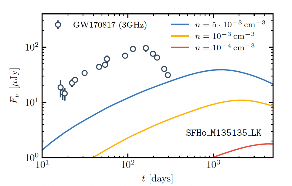
Fig 4. Radio light curves of the dynamical ejecta of one model at 3 GHz, compared with GW170817. The ISM number density n is a parameter of the model used for generating the curves. [Radice et al. 2018]
Looking Ahead
Systematic investigations are key to understanding complex events such as neutron-star mergers. Improved theoretical modeling, with a push towards incorporating all the relevant physics in merger models, will not only help us understand what we saw last year but also set us up for the next set of observations!
About the author, Sanjana Curtis:
I’m a grad student at North Carolina State University. I’m interested in extreme astrophysical events like core-collapse supernovae and compact object mergers.


 Gaps in our Knowledge of Planet Formation")