Cepheid Yourself: Confirming Tensions in the Hubble Expansion
Editor’s note: Astrobites is a graduate-student-run organization that digests astrophysical literature for undergraduate students. As part of the partnership between the AAS and astrobites, we occasionally repost astrobites content here at AAS Nova. We hope you enjoy this post from astrobites; the original will be viewable at astrobites.org once the site has been fully restored.
Title: Large Magellanic Cloud Cepheid Standards Provide a 1% Foundation for the Determination of the Hubble Constant and Stronger Evidence for Physics Beyond ΛCDM
Authors: Adam G. Riess, Stefano Casertano, Wenlong Yuan, Lucas M. Macri, Dan Scolnic
First Author’s Institution: Space Telescope Science Institute and Johns Hopkins University
Status: Published in ApJ
Hubble’s law tells us that all galaxies, stars and planets are moving away from each other, and the more distant the object, the faster it is moving away. We quantify this expansion as a speed per distance, which gives us a unit like km/s (speed) per megaparsec (distance). This value is known as the Hubble constant, or H0.
The Hubble constant has been determined using various methods. However, two of these titan measurements disagree with each other in a way that astronomers deem significant.
The first of the measurements comes from studying the oldest electromagnetic radiation in the universe — the cosmic microwave background (CMB). See this Astrobite for a detailed explanation of how we are able to do this. The most recent results from the CMB give us a Hubble constant of roughly 67 km/s/Mpc.
The second measurement comes from using Type Ia supernovae as standard candles to calibrate distances to them (see this Astrobite for more). Essentially, by looking at these stars at various distances, we can correlate their distance with their apparent brightness. By assuming supernovae are dimmer proportional to their distance from us, we can measure the gradient of this correlation. Recent results put H0 at 73 km/s/Mpc.
So, one of the most prominent problems in cosmology boils down to a 6 km/s/Mpc difference. Certainly, each of these measurements have their own subtleties but there are two main things to note:
- The Hubble-constant measurements using the CMB and Type Ia supernovae are independent. They do not rely on the same measurement technique, and therefore do not have any source of error in common. This makes it harder to dismiss the tension as something which comes from a shared, inaccurate measurement.
- The Hubble-constant measurement from the CMB uses data from the early universe, while the value obtained from supernovae is a late-time or local measurement. This could potentially be an interesting explanation for the tension.
A New Addition
Today’s authors stir the Hubble cauldron a bit more with 70 space-based observations of Cepheid variables in the Large Magellanic Cloud (LMC) from the Hubble Space Telescope.
A Cepheid variable is a type of star that pulsates over some period of time. Astronomer Henrietta Swan Leavitt deduced that the rate of pulsation for these stars is correlated strongly with their luminosity (see this Astrobite for more on her work and legacy). Therefore, one can know the brightness of these stars simply by observing their pulsation rate (Figure 1). Consequently, one can determine the distance to these stars just by comparing their known luminosity to the apparent brightness. Much like supernovae, this makes Cepheid variables powerful probes of the local Hubble constant. Furthermore, by studying galaxies containing both Cepheid variables and type Ia supernovae, the Cepheid-derived distances can be used to calibrate the accuracy of supernovae-derived distances, creating a robust distance ladder, which gets us to H0.
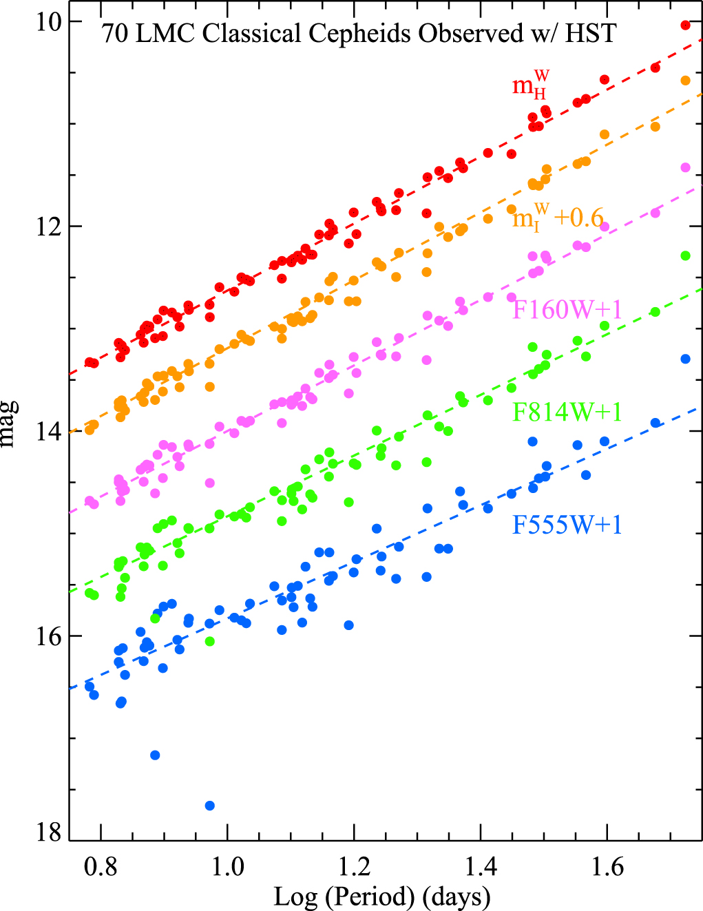
Figure 1: Period-luminosity relation for the 70 Cepheid variable stars. The colours in the figure indicate the different wavelengths used for observing these Cepheids. The agreement in the slope tells us the P–L relation is not dependent on any particular wavelength. [Riess et al. 2019]
So What’s the Tension Now?
Combining the LMC distances with two other distance calibrators for better constraints, the authors quote a Hubble constant of 74.03 km/s/Mpc, which is in a staggering 4.4-σ tension with the CMB Hubble-constant measurement. This effectively means that the probability that the new measurement is genuine rather than a statistical fluke is above 99.999%, and therefore so is the discrepancy.
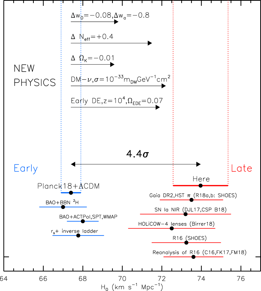
Figure 2: Various measurements of the Hubble constant colour-coded by whether they use data from the early universe (blue) or the late universe (red). At the top are potential modifications to our current cosmological model which could resolve the current tension. [Riess et al. 2019]
About the author, Sunayana Bhargava:
I’m a third year PhD student in the Astronomy Centre at the University of Sussex. I study galaxy clusters with X-ray and optical data to learn about cosmology and the properties of dark matter.


 Light Up My Life")

