A New Site for the s-Process?
Editor’s note: AAS Nova is on vacation this week. Normal posting will resume next week; in the meantime, we hope you enjoy this post from Astrobites, a graduate-student-run organization that digests astrophysical literature for undergraduate students. The original can be viewed at astrobites.org.
Title: New s-process Site in Rapidly-Rotating Massive Pop II Stars
Authors: Projjwal Banerjee, Alexander Heger, Yong-Zhong
First Author’s Institution: Indian Institute of Technology Palakkad, India; Shanghai Jiao Tong University, China
Status: Submitted to ApJ
One of the main goals of nuclear astrophysics is to understand and explain the composition of the universe. Starting out with hydrogen, helium, and a teeny bit of lithium, the universe evolved to have an entire periodic table worth of chemical elements. How did this happen? We know that stars and supernovae played a key role in this chemical enrichment. However, exactly how and where different elements are produced, and in what quantities, remains a topic of vigorous ongoing research. Heavy element nucleosynthesis is a key piece of this puzzle and has received a lot of attention recently in the context of neutron star mergers.
Heavy elements — i.e., elements heavier than iron — are mainly formed through the s-process and the r-process. The names describe the speed of the process relative to the decay time of the isotopes involved: s-process involves slow neutron capture and the r-process involves rapid neutron capture.
Although both these processes make roughly equal overall contributions to the total abundance of heavy elements, the s-process does not get the same hype as its cool twin, the r-process. This is partly due to the fact that the site of the r-process was a huge mystery until very recently, when neutron star mergers were identified as one of the sites where the process occurs. It still remains to be seen whether they are the only site of the r-process.
The s-process, on the other hand, is known to occur inside asymptotic giant branch (AGB) stars. This is the final stage of evolution for long-lived, low-mass stars between 1–3 solar masses. The AGB stars can produce elements up to 209Bi, forming what’s called the “main” component of the s-process. However, a weaker version of the s-process also happens in massive stars (>10 solar masses), producing elements up to atomic mass number A ~ 90. Today’s paper shakes things up by introducing a new site for the main s-process: in rotating metal-poor massive stars!
The authors find that above a critical rotation speed, massive metal-poor stars evolve in a quasi-chemically-homogeneous (QCH) manner. This means the stars are spinning so fast that the mixing caused by rotation becomes very efficient. At the end of core hydrogen-burning, which produces helium, these stars look like helium stars. We can see this in panel (a) of Figure 2. Now starts the story of the s-process, which goes like this:
- The star in the QCH state starts burning helium in the center, producing 12C. Its core becomes convective.
- The convective core grows in size. Some of the 12C is mixed outward into the radiative region of the star. In this region, there are still some protons present, along with the right thermodynamic conditions to allow 12C to react with protons. This produces 13C.
- Some 13C is mixed back into the convective He-burning core. In regions that are hot enough, 13C reacts efficiently with the 4He, producing oxygen, as well as neutrons. This leads to high neutron densities that allow the s-process to happen!
We can see this play out in panels (b) through (d) of Figure 1.
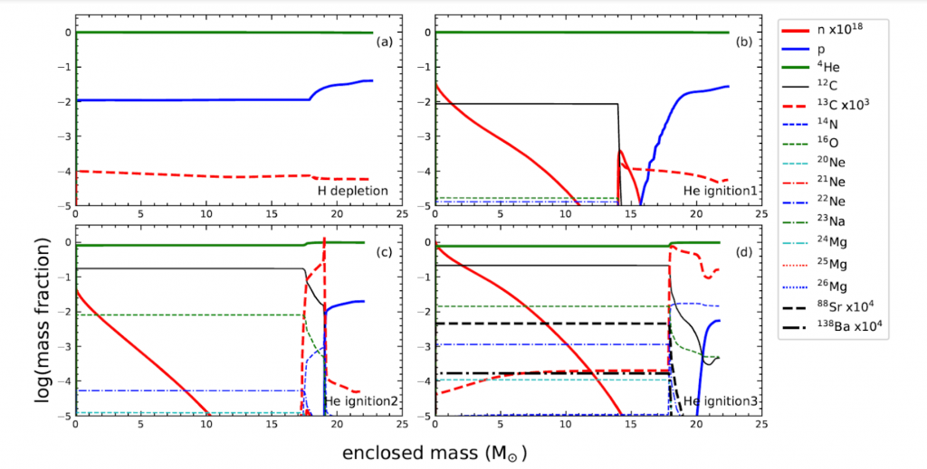
Figure 1. Isotopic composition of the star during different stages of its evolution. The y-axis gives the mass fraction of different isotopes and the x-axis indicates the mass coordinate, i.e., how much mass of the star we’re looking at as we move away from the center of the star. We can see the mass fraction of 13C growing as 12C gets mixed into and reacts with protons in the outer layers. This 13C gets mixed inward and reacts with 4He, producing both 16O and neutrons. [Banerjee et al. 2019]
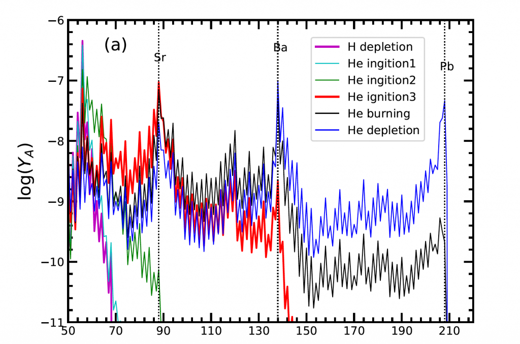
Figure 2. Time evolution of the s-process yield pattern for a 25-solar-mass star. Number yields of heavy isotopes inside the star are plotted as functions of mass number. The different lines correspond to different stages in the star’s evolution. [Banerjee et al. 2019]
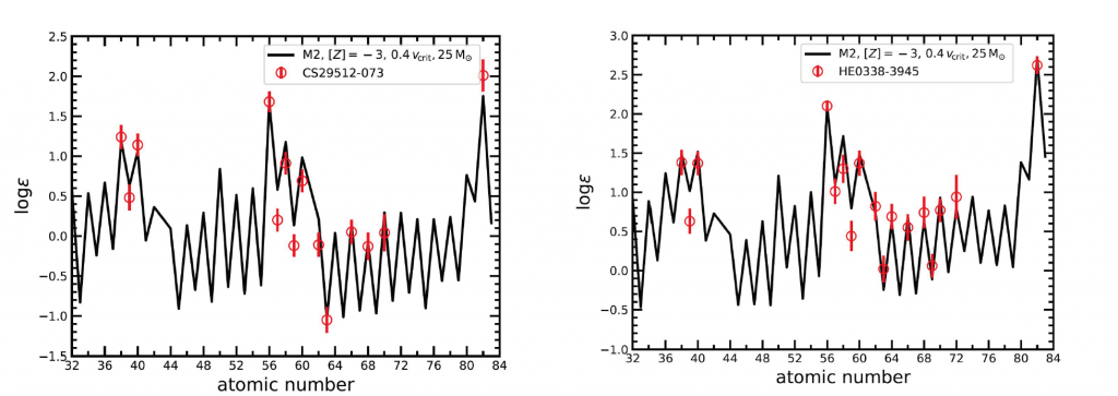
Figure 3. Heavy-element abundances from this work compared to VMP stars. The abundances are from the wind ejecta (left) and the wind ejecta combined with outer stellar ejecta (right) for a 25-solar-mass star. The stars shown here are CEMP stars. The one on the left is a CEMP-s star while the one on the right is a CEMP-r/s star. [Adapted from Banerjee et al. 2019]
About the author, Sanjana Curtis:
I’m a grad student at North Carolina State University. I’m interested in extreme astrophysical events like core-collapse supernovae and compact object mergers.