
Plenty of Gas Left in Giant Dead Disk Galaxies
Editor’s note: Astrobites is a graduate-student-run organization that digests astrophysical literature for undergraduate students. As part of the partnership between the AAS and astrobites, we occasionally repost astrobites content here at AAS Nova. We hope you enjoy this post from astrobites; the original can be viewed at astrobites.org.
Title: Nearly all Massive Quiescent Disk Galaxies have a Surprisingly Large Atomic Gas Reservoir
Authors: C. Zhang et al.
First Author’s Institution: Peking University, China
Status: Published in ApJL
A concept fundamental in astronomy is that stars form from cold, dense molecular gas clouds. Applied to the formation and evolution of galaxies, star-formation is understood as being directly supported by an abundance of this cold molecular gas. We find that in star-forming galaxies — typically disk-like with blue spiral arms — there is a large reservoir of this cold molecular gas from which rapid star-formation can be sustained. Quiescent galaxies, on the other hand — typically elliptical-like with red colors — do not actively form stars. Hence, they have been long thought to have only a scarce supply of cold molecular gas, likely as a result of either vigorous star-formation in the past, some sort of gas reservoir removal event, or a combination of the two.
There is overwhelming evidence that star-forming and quiescent galaxies inhabit very different environments in our universe. While star-forming galaxies are generally found alone or in small groups, quiescent galaxies are often found residing in large galaxy clusters with tens to hundreds of cluster members. This so-called morphology-density relation tells us something fundamental about the role of environment in shaping galaxy properties. In particular, it suggests that the cluster environment influences the ceasing (or quenching) of star-formation.
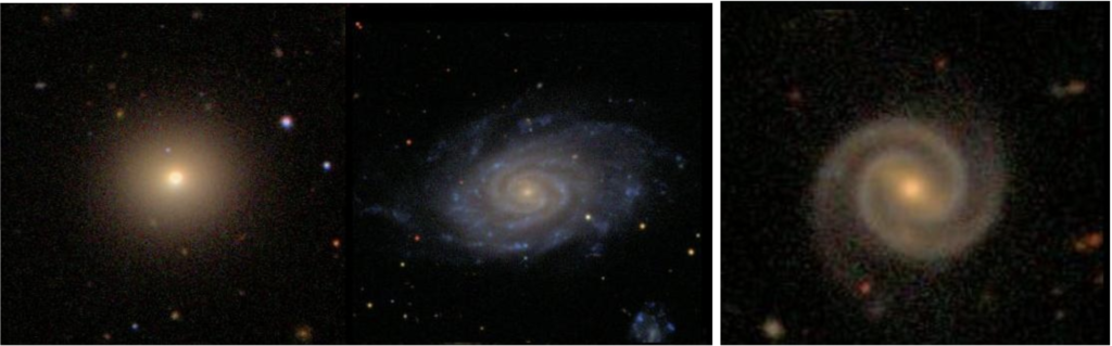
Figure 1. Archetypal quiescent elliptical galaxies (left) and star-forming spirals (middle) comprise the vast majority of galaxy demographics. Rare and poorly understood red disk spirals remain a puzzling mystery (right). [Masters et al. 2010]
Today’s paper discusses new and surprising findings about the gas content of these massive central galaxies, and how the galaxies are kept from forming stars.
A statistically large sample of nearby massive central galaxies was carefully selected from the Sloan Digital Sky Survey (SDSS). Instead of focusing on just typical giant central galaxies that have elliptical morphologies, the authors chose to examine the ellipticals side-by-side with little-appreciated massive central disk galaxies. These kinds of galaxy cross-breeds are extremely rare, but potentially interesting objects for understanding the complex and poorly understood mechanisms that drive star-formation cessation. Morphological classifications of elliptical and disk galaxies were taken from the citizen science project Galaxy Zoo, which crowd-sources galaxy classification through an online web platform accessible to anyone.
However, the SDSS data is only half the story. The SDSS galaxies were crossed matched with deep centimeter-wavelength surveys (ALFALFA and GASS) in order to obtain measurements of the atomic gas (H I) in these galaxies. While the atomic gas is too hot to directly form stars, given the right conditions it may cool down into molecular gas (H2).
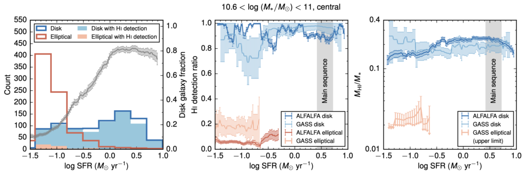
Figure 2. (Left) the distribution of massive elliptical and disk central galaxies, with the fractional abundance of disk galaxies shown in grey. (Middle) the strength of H I detection as a function of star-formation rate for disk and elliptical central galaxies. (Right) Similarly, the atomic gas mass. [Zhang et al. 2019]
Importantly, this implies that massive quiescent central disk galaxies do indeed have the raw gas supply necessary to form stars. The lack of star formation then must either be due to a marked inefficiency in converting atomic gas into molecular gas, difficulty in forming stars from the molecular gas, or both.
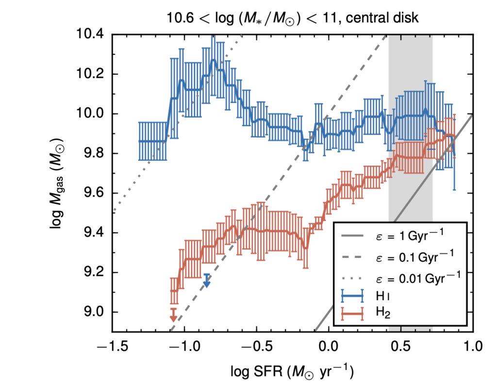
Figure 3. Atomic (red) and molecular (blue) gas mass as a function of star-formation rate in massive central disk galaxies. [Zhang et al. 2019]
Taken together, this investigation into the gas content of massive central disk galaxies illustrates that although their atomic gas content is universally large compared to central ellipticals, their star-formation cessation is still driven by a dearth of cold molecular gas. Yet, the precise mechanism keeping the atomic gas from eventually giving way to star formation remains elusive.
About the author, John Weaver:
I am a second year PhD student at the Cosmic Dawn Center at the University of Copenhagen, where I study the formation and evolution of galaxies across cosmic time with incredibly deep observations in the optical and infrared. I got my start at a little planetarium, and I’ve been doing lots of public outreach and citizen science ever since.


