How It’s Made, Fast Radio Burst Edition
Editor’s note: Astrobites is a graduate-student-run organization that digests astrophysical literature for undergraduate students. As part of the partnership between the AAS and astrobites, we occasionally repost astrobites content here at AAS Nova. We hope you enjoy this post from astrobites; the original can be viewed at astrobites.org.
Title: Spectropolarimetric analysis of FRB 181112 at microsecond resolution: Implications for Fast Radio Burst emission mechanism
Authors: Hyerin Cho et al.
First Author’s Institution: Gwangju Institute of Science and Technology, Korea
Status: Published in ApJL
Fast radio bursts (FRBs) are probably the fastest growing and most interesting field in radio astronomy right now. These extragalactic, incredibly energetic bursts last just a few milliseconds and come in two flavors, singular and repeating. Recently the number of known FRBs has exploded, as the Canadian Hydrogen Intensity Mapping Experiment (CHIME) radio telescope has discovered about 20 repeating FRBs (and also redetected the famous FRB 121102) and over 700 single bursts (hinted at here). However, despite the huge growth in the known FRB population, we still don’t know what the source(s) of these bursts is (are). Today’s paper looks at possible explanations for the properties of one FRB in particular to try to figure out what its source might be.
Your Friendly Neighborhood FRB
A number of previous astrobites have discussed the basics of FRBs (here, here, and here for example) but the FRB that the authors of this paper focus on is FRB 181112. FRB 181112 was found with the Australian Square Kilometer Array Pathfinder (ASKAP) and localized to a host galaxy about 2.7 Gpc away from us even though it has not been observed to repeat. That’s over a hundred times farther away than the closest galaxy cluster, the Virgo Cluster! One quality of FRB 181112 that makes it particularly interesting to study is that the way ASKAP records data allows the authors to study the polarization of the radio emission. Polarization of light is a measure of how much the electromagnetic wave (here the radio emission) rotates due to any magnetic fields it propagates through. The two types of polarization are linear polarization (Q for vertical/horizontal, or V for ±45°), which occurs if the electromagnetic wave rotates in a plane, and circular (either left- or right-handed depending on the rotation direction) if the light rotates on a circular path. By looking at the polarization of FRB 181112, shown in Figure 1, the authors can determine the strength of the magnetic field it traveled through.
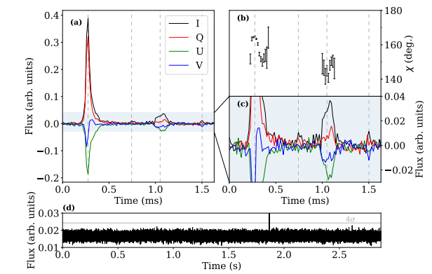
Figure 1: a) The full polarization profile of FRB 181112 showing four profile components. The black line, I, is the sum of all the polarizations of light, or the total intensity of the burst. The red line, Q, is the profile using only (linearly) horizontally or vertically polarized light; the green line, U, is using only the (linearly) ±45° polarized light; and the blue line, V, is the profile using only circularly polarized light. Negative values describe the direction of the polarization. b) The polarization position angle of the zoomed in profiles from panel (a) seen in panel (c). Variation here suggests the emission is coming from different places in the source. d) A three second time series of the data where the FRB is clearly visible at about 1.8 seconds. [Cho et al. 2020]
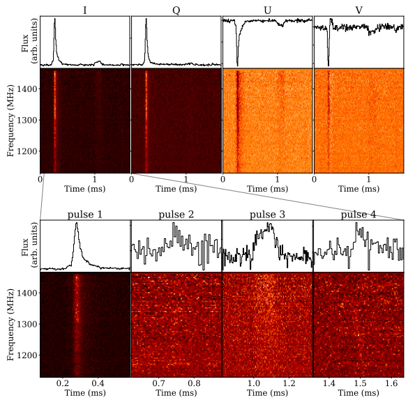
Figure 2: Top row: Intensity of the radio emission of each of the four polarization profiles, I, Q, U, and V (described in Figure 1) as a function of time and radio frequency. Bottom row: Close up of the four different pulse components of the total intensity polarization profile, I, of FRB 181112 as a function of time and radio frequency. All components have been assumed to have a DM of 589.265 pc cm-3 , and a slight slope in the intensity as a function of time and frequency can be seen in pulse 4, indicating it may have a slightly different DM. [Cho et al. 2020]
Properties of FRB 181112
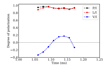
Figure 3: Degree of polarization of FRB 181112. The black line (P/I) shows the total polarization, the red line (L/I) shows the linear polarization, and the blue line (V/I) shows the circular polarization. The red and black lines show a large amount of polarization constant in time, while the blue line shows the circular polarization changes over the pulse. [Cho et al. 2020]
The authors next analyzed the four different components shown in the bottom row of Figure 2 for variations in DM and find there are some small, but significant differences between each component. These differences could be due to some unmodeled structure in the ISM, again possibly a relativistic plasma, but is unlikely since the burst lasts for only 2 milliseconds. The authors also suggest these differences in DM could be due to gravitational lensing, the radio light being bent around a massive object. This would mean different components travel through different paths in the ISM, accounting for the different DMs and four different components. However, gravitational lensing cannot explain the high degree of polarization seen in FRB 181112.
The Million Dollar Question
So how was FRB 181112 made? What caused the polarization and differences in DM? Well, the authors can’t say anything for certain. They suggest that the most likely model is a relativistic plasma close to the source of the emission, which has polarization properties similar to known magnetars (highly magnetized neutron stars known to emit radio bursts), but none of their models can fully explain all of the different properties of FRB 181112. The source of FRB 181112 remains a mystery for now, but with the huge number of FRBs now being detected, the answer may lie just around the corner.
About the author, Brent Shapiro-Albert:
I’m a fourth year graduate student at West Virginia University studying various aspects of pulsars. I’m a member of the NANOGrav collaboration which uses pulsar timing arrays to detect gravitational waves. In particular I study how the interstellar medium affects the pulsar emission. Other than research I enjoy reading, hiking, and video games.

 Ships")