Features RSS

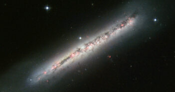
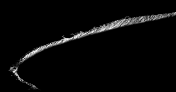
A photograph of a galaxy which appears in the foreground as a diagonal line because of the edge-on viewing geometry.

In the early universe, galaxies were misshapen blobs that could only dream of transforming into something as structured and stately as our present Milky Way. Unfortunately, pinning down exactly when in history some early galaxies flattened into disks is a challenging task; now, though, the formidable combination of JWST and deep learning offers steps towards an answer.

Challenging Finds

When do disky galaxies form? In theory, answering this question is straightforward: astronomers just need to look back in time, which they (somewhat remarkably) can do by looking at higher and higher redshifts, and see when disks first appear. Unfortunately but unsurprisingly, what’s simple in description is difficult in practice. High-redshift galaxies appear extremely faint in visible light and instead are brightest in the infrared, which historically was much harder to detect with high-spatial-resolution detectors. Although the Hubble Space Telescope was a transformative telescope in so many ways, it struggled to find or resolve many high-redshift galaxies.

Enter JWST. It was designed in part to find these evasive galaxies: its detectors all are sensitive to longer wavelengths of light, and especially its NIRCam instrument is expected to be a workhorse of galaxy discovery and classification. This work has already begun in earnest, and several of the observations associated with the Cosmic Evolution Early Release Science Survey (CEERS) have already been taken.

Finding Disks

Images taken by JWST of a CEERS field. Along the top and bottom are rows of inset frames which magnify specific galaxies in the image. The magnified images show generally extended disk-like shapes, but are heavily blurred/pixelated given the small angular size of these targets.

False-color JWST images and a selection of galaxies that Morpheus classified as “disky.” The photometric redshift of each galaxy is noted in the upper corner of each inset. [Robertson et al. 2023]

Though the CEERS team is still hard at work on their analysis, their data were made public immediately to allow other researchers to take a look. This allowed a collaboration led by Brant Robertson (University of California, Santa Cruz) to run their own analysis tools on a series of images taken of a region called the Extended Groth Strip.

The tool they deployed was a deep learning model named Morpheus, which back in 2020 was trained to ingest images taken by Hubble, spot high-redshift galaxies, and then classify them according to their morphology. In that earlier study, the authors compared how many galaxies were “disks” vs. “spheroids” (and other categories) at different redshifts to estimate when structure first emerged. With JWST images in hand of the exact same patch of sky, they played the same game on the same galaxies with the new data and compared the results.

A 3 row, 4 column panel figure. From left to right, the columns are labeled "Morpheus", "JWST/F150W", "Model", and "Residual". Each row corresponds to a different example galaxy, and when read across left to right demonstrates Morpheus's ability to build a model which accurately matches the data.

An example of Morpheus’s classification “under the hood.” The network assigns a probability to each pixel that it belongs to a certain galaxy classification, then assigns a classification for any object that has >50% probability of being in a certain class. [Robertson et al. 2023]

In this first-ever application of AI/ML tools to JWST data, the authors cross-matched >7,000 galaxies between the Hubble and JWST images, and interestingly, noticed that Morpheus changed its mind about how to classify some of the faintest and highest-redshift targets. Of the 160 faintest (H>24.5AB!) galaxies Morpheus claimed were disk galaxies after seeing the JWST images, it had previously only thought 5% were flat in the Hubble data. Most of the others were too faint to resolve at those shorter wavelengths, so they had previously been mislabeled as “compact,” point-like sources, when in fact there was some structure Hubble had simply missed. Excitingly, some of the newly-classified disk galaxies have photometric redshifts of 4-5, a surprisingly high value which will require further analysis to fully contextualize.

While it’s still too early for any precise estimates of the disk formation timescale, these results confirm that JWST is a transformative tool for the job. Now more than a year since launch, we can be sure to expect more galaxies, more accurate classifications, and more rewrites to our current understanding of galaxy formation in short order.

Citation

“Morpheus Reveals Distant Disk Galaxy Morphologies with JWST: The First AI/ML Analysis of JWST Images,” Brant E. Robertson et al 2023 ApJL 942 L42. doi:10.3847/2041-8213/aca086

JWST image of the galaxy cluster SMACS 0723

In the months since the release of the first JWST image of the galaxy cluster SMACS J0723.3–7327 (SMACS 0723), astronomers have studied the image from every possible angle. Today’s post takes a look at five research articles that have advanced our understanding of galaxies within the cluster and beyond.

How to Weigh a Cluster

SMACS 0723 is a galaxy cluster located four billion light-years away. It gets its name from the Southern MAssive Cluster Survey (SMACS), in which the Hubble Space Telescope observed 124 galaxy clusters that are bright at X-ray wavelengths. In addition to the galaxies bound to the cluster, observations of SMACS 0723 contain images of galaxies far more distant. This is because SMACS 0723 is so massive that it warps spacetime, causing photons from galaxies billions of light-years away to curve around the foreground galaxies and into our field of view. As a result, we see stretched-out, wiggly, or multiple images of distant galaxies.

two mass density distribution maps for galaxy cluster SMACS 0723

Top: Mass distribution derived by Mahler and collaborators. The magenta lines are mass contours and the white lines are X-ray surface brightness contours. Bottom: Mass distribution derived by Pascale and collaborators. The black lines show the surface mass density distribution. Note that there is a difference in scale and orientation between the two maps. [Adapted from Mahler et al. 2023; Pascale et al. 2022]

Researchers can use these wiggly galaxies to reconstruct a map of SMACS 0723’s mass distribution. Understanding how a cluster’s mass is distributed is important because it can tell us about the underlying distribution of dark matter within the cluster and how the cluster has evolved over time. As is often the case when exciting new data are released, several teams worked in parallel to map SMACS 0723’s mass distribution using different techniques. Two articles published in AAS journals detail efforts by teams led by Massimo Pascale (University of California, Berkeley) and Guillaume Mahler (Durham University) to use JWST’s superior capabilities to improve upon the existing mass map based on Hubble data.

In previous observations of the cluster, astronomers picked out five lensed background galaxies, but JWST’s impressive capabilities allowed the teams to pick out many more; at 6.5 meters in diameter, JWST is already a massive space telescope, but as Pascale and coauthors noted, pointing it toward a galaxy cluster that bends the light from more distant sources effectively creates a telescope with a diameter of 20–30 meters!

Pascale’s and Mahler’s teams used different computer algorithms to analyze the lensed galaxies newly identified in the JWST images, and both teams achieved a large increase in the precision of their mass maps compared to those based on Hubble data. Both teams’ maps show evidence of a past disturbance in the galaxy cluster, such as gravitational interactions or mergers between galaxies.

A Trio of Distant Galaxies

Karla Arellano-Córdova (The University of Texas at Austin) and collaborators took advantage of SMACS 0723’s lensing ability to study three galaxies with redshift, z, between 7.6 and 8.5, corresponding to when the universe was about 600–700 million years old. Using JWST’s Near-Infrared Spectrograph (NIRSpec), the team identified emission lines in the spectra of these distant galaxies. By measuring the strength of several prominent emission lines and the ratios of their strengths relative to one another, Arellano-Córdova’s team determined the properties of the gas in each galaxy, including the abundance of elements like carbon, oxygen, neon, and potentially iron. Notably, the team measured the neon-to-oxygen abundance ratio for a galaxy at z > 7 for the first time, and they obtained the most distant carbon-to-oxygen ratio measurement ever.

metallicity versus stellar mass for star-forming galaxies

Metallicity versus stellar mass for galaxies in the local universe (light blue circles) and at high redshift. Values from this work are shown with stars, while other researchers’ results are shown with triangles, diamonds, pentagons, and squares. [Arellano-Córdova et al. 2022]

By comparing the chemical abundances for the three high-redshift galaxies to those of nearby galaxies, the team gained a sense of how each element’s abundance has changed over time, which can inform us about how galactic stellar populations evolved early in the universe. While some of the abundances followed expected trends, others showed behavior that will require further inspection; a tentative detection of emission lines from iron atoms suggests that these galaxies might be rich in iron compared to oxygen, which the authors propose could be due to gaseous outflows. The authors emphasized that this is just the beginning of what JWST will accomplish in terms of investigating the chemical makeup of galaxies in the first billion years of the universe — we’ve cracked open a window into that time period, and future studies should open it wider still.

Investigating Point Sources in SMACS 0723

The final two articles focus on goings on within the cluster itself, using JWST’s exceptional precision to investigate individual star clusters four billion light-years away.

several panels illustrating the locations of the star clusters within the SMACS 0723 field

Location of the star clusters studied in this work within the larger SMACS 0723 field. Click to enlarge. [Faisst et al. 2022]

A team led by Andreas L. Faisst (California Institute of Technology — Infrared Processing and Analysis Center) searched the SMACS 0723 images for signs of star clusters. The team manually selected 178 promising sources from the images, finding that the human eye was better at picking out the faint clusters against the background galactic light than a search algorithm. Because the individual star clusters were so faint, the team combined the measurements for all 178 clusters to determine the average properties of the sample.

Overall, the clusters appear to be about 1.5 billion years old, although the team could not rule out the possibility that the clusters are up to 9 billion years old (roughly the age of the universe at SMACS 0723’s redshift). Given the clusters’ sizes (no more than 160 light-years across), masses (about 2.4 million solar masses, on average), and metallicity (about 20–30% the metal abundance of the Sun), the team concluded that the star clusters are most likely to be globular clusters: roughly spherical collections of hundreds of thousands of stars found on the outskirts of nearly all galaxies. However, the authors acknowledged another possibility: as dwarf galaxies surf the gravitational swells of the massive galaxy cluster where they were born, they may lose their outermost stars, resulting in dense star clusters similar to those seen in SMACS 0723.

Galaxy Cluster Globular Clusters

Myung Gyoon Lee (Seoul National University) and collaborators also went globular cluster–hunting in the SMACS 0723 images, using an algorithm to identify and characterize point sources throughout the galaxy cluster. By grouping point sources based on their color and brightness, the team identified those that are most likely to be globular clusters associated with the SMACS 0723 galaxy cluster.

illustration of the locations of the sources studied in this work

Illustration of the location of some of the sources studied in this work. Click to enlarge. [Lee et al. 2022]

Many of the sources appear to be linked to the brightest galaxy in the cluster, which lies near the cluster center. These star clusters are most concentrated near the bright central galaxy and become more scattered farther out, and similar concentrations are seen around other bright galaxies within the cluster.

In addition to tracing the distribution of galaxies in SMACS 0723, the candidate globular clusters also follow some of the intracluster structures, such as the distribution of diffuse intracluster light. This faint emission comes from stars that have been ejected from their home galaxy due to gravitational interactions between galaxies in the cluster. The team also compared the star cluster distribution to the dark matter distribution determined in other research articles, finding considerable similarities between the two distributions. These findings suggest that star clusters can be used to trace dark matter within galaxy clusters.

Citation

“Unscrambling the Lensed Galaxies in JWST Images behind SMACS 0723,” Massimo Pascale et al 2022 ApJL 938 L6. doi:10.3847/2041-8213/ac9316

“Precision Modeling of JWST’s First Cluster Lens SMACS J0723.3–7327,” Guillaume Mahler et al 2023 ApJ 945 49. doi:10.3847/1538-4357/acaea9

“A First Look at the Abundance Pattern—O/H, C/O, and Ne/O—in z > 7 Galaxies with JWST/NIRSpec,” Karla Z. Arellano-Córdova et al 2022 ApJL 940 L23. doi:10.3847/2041-8213/ac9ab2

“What Are Those Tiny Things? A First Study of Compact Star Clusters in the SMACS0723 Field with JWST,” Andreas L. Faisst et al 2022 ApJL 941 L11. doi:10.3847/2041-8213/aca1bf

“Detection of Intracluster Globular Clusters in the First JWST Images of the Gravitational Lens Cluster SMACS J0723.3–7327 at z = 0.39,” Myung Gyoon Lee et al 2022 ApJL 940 L19. doi:10.3847/2041-8213/ac990b

a representation of the Sun's spectrum

Solar physicists have identified the best way to measure magnetic fields in the solar atmosphere, opening the door to deciphering the mysteries of a poorly understood part of the Sun.

An illustration of the regions of the Sun's atmosphere and interior.

An illustration of the regions of the Sun’s atmosphere and interior. Click to enlarge. [NASA/Goddard]

Our Multilayered Star

The Sun’s atmosphere has three layers: the photosphere, the chromosphere and the corona. The photosphere is the Sun’s visible surface and the corona is the wispy, tenuous outermost layer visible during solar eclipses. The chromosphere, a name that means sphere of colour, is sandwiched between the two and is incredibly thin. It takes up just one per cent of the Sun’s radius and yet understanding it is important work.

Strong magnetic fields corral hot plasma in the chromosphere into a network of super-sized granulation cells that can stretch to 20,000 miles across — some 2.5 Earth diameters — and 1,000 miles deep. On the edges of the cells sit spicules: spikes of magnetically confined plasma that shoot up into the corona above. The release of magnetic energy is also linked to events such as solar flares and coronal mass ejections, which can cause issues for our electrical infrastructure on Earth. So solar physicists want to know how magnetic fields emerge from, heat, and accelerate chromospheric plasma.

Magnetic Field Measurement

One way to measure the magnetic fields in the chromosphere is to take advantage of the Zeeman effect. Strong magnetic fields split the lines observed in the Sun’s spectrum. Recently a team led by Philip Judge (National Center for Atmospheric Research, Colorado) did something no one had ever done before: assess the comparative merits of using all spectral lines from X-ray to infrared wavelengths to measure magnetic fields as high as possible in the solar atmosphere.

an example solar spectrum

A sample solar spectrum with prominent spectral lines labeled. Click to enlarge. [Judge et al. 2022]

The team concluded that the best lines for the job are the magnesium h and k lines near 2800 Ångstroms (Å). However, they also found that combining them with the numerous chromospheric lines of iron between 2585 Å and the h line at 2803 Å would provide a far more discriminating probe of magnetic structure in the chromosphere. All of these wavelengths sit in the ultraviolet part of the spectrum.

Future Prospects

The recent Chromosphere Lyman-Alpha Spectro-Polarimeter (CLASP-2) instrument launched aboard a sounding rocket demonstrated that measurements at these wavelengths can be made successfully. A modest space-borne telescope focussing on the same part of the spectrum could provide a way to untangle some of the biggest riddles about the Sun’s chromosphere and the violent eruptions associated with it.

Citation

“Optimal Spectral Lines for Measuring Chromospheric Magnetic Fields,” P. Judge et al 2022 ApJ 941 159. doi:10.3847/1538-4357/aca2a5

artist's impression of a kilonova explosion

Astronomers are still debating the origin of the blue-tinted emission from colliding neutron stars detected in 2017. Stymied by missing data from the crucial first few hours of that event, researchers have determined just how quickly we’ll need to catch the next one.

A Groundbreaking Event

light curves for the electromagnetic counterpart to a gravitational wave signal detected in August 2017

Observed (symbols) and modeled (lines) light curves for AT2017gfo, the electromagnetic counterpart to the gravitational wave signal GW170817. [Adapted from Cowperthwaite et al. 2017]

In August 2017, a pair of gravitational wave detectors identified a signal from two neutron stars — the ultra-dense remnants of massive stars — colliding 130 million light-years away. In the hours that followed, a network of telescopes raced to search for the electromagnetic counterpart to the event (dubbed AT2017gf), with telescopes locking on to the source 11 hours after the merger was detected.

These observations revealed bright but rapidly fading emission at blue wavelengths in the first day after the collision was detected. Though scientists have proposed many causes for this early blue emission, two theories have risen to the top: radioactive decay of newly fused elements and heating from a shock wave. Researchers suspect that in order to distinguish between these theories, we need ultraviolet data from the first few hours after the merger is detected. We missed those critical data in 2017, with ultraviolet observations beginning 15 hours after detection — how can we ensure we capture them in the future?

When Theories Collide

Bas Dorsman (University of Amsterdam) and collaborators proposed that an ultraviolet satellite with a wide field of view could capture the necessary data next time around. To test this possibility, the team modeled the emission from an AT2017gfo–like collision of two neutron stars, finding that both theories produce ultraviolet emission that matches observations at 15 hours after the event was detected but diverges at earlier times.

plot of simulated light curves for the two competing theories

Simulated ultraviolet light curves for an AT2017gfo–like neutron star merger. The orange and green lines show the results for two versions of the radioactive decay model, the blue line shows the output from the shock heating model, and the gray line shows the time at which the ultraviolet observations of AT2017gfo began. [Dorsman et al. 2023]

To estimate just how quickly we’d need to begin collecting ultraviolet data to draw firm conclusions, Dorsman and coauthors considered the capabilities of a proposed ultraviolet satellite called Dorado. Using their model results, the team simulated what a Dorado-like spacecraft would detect during the early hours of an AT2017gfo–like event. Ultimately, they found that if the ultraviolet data collection starts 1.2 hours after the event is detected — the best-case scenario based on the satellite’s capabilities — we’d be able to distinguish between the two theories for events within about 522 million light-years of Earth. As the time of first observation grows later, the events need to be closer for us to tell what drives the early blue emission: out to 424 million light-years for data starting at 3.2 hours and out to 196 million light-years for data starting at 5.2 hours.

Awaiting Spacecraft

While the team’s results show the promise of collecting early ultraviolet data, we’ll need to wait at least a few years to put the plan into practice. The Dorado spacecraft described in this work didn’t proceed beyond a concept study, but there are two similar spacecraft farther along in the selection process: the Ultraviolet Transient Astronomy Satellite (ULTRASAT; launch planned for 2026) and the Ultraviolet Explorer (UVEX; launch in 2027 or later, if selected).

These missions should overlap with the fifth observing run for the LIGO, Virgo, and KAGRA gravitational wave observatories, which is slated to begin in 2027. Hopefully — a decade after the detection of AT2017gfo — we’ll be able to get some answers!

Citation

“Prospects of Gravitational-wave Follow-up through a Wide-field Ultraviolet Satellite: A Dorado Case Study,” Bas Dorsman et al 2023 ApJ 944 126. doi:10.3847/1538-4357/acaa9e

A photograph of a building and other infrastructure atop an ice sheet at night. Several stars are visible overhead.

The universe is crackling with gravitational waves and sparkling with neutrino emissions, but detecting both signals from the same source is an enormous challenge. A new publication summarizes the state of this effort and reports on non-detections of high-energy neutrinos associated with the merger events caught by LIGO/Virgo.

Multiple Messengers

Historically, astronomers studied our universe by analyzing the electromagnetic radiation (light) that lands on Earth after a journey through the depths of the cosmos. In the last decade, however, researchers have expanded upon this paradigm and now routinely scrutinize other “messengers” that collide with our home planet and leave their imprints on our scientific instruments. Two of these messengers include high-energy neutrinos, first observed in 2013, and gravitational waves, first spotted in 2015.

Certain astrophysical processes, including the mergers of compact objects like black holes and neutron stars, are thought to produce both of these messengers. Therefore, to wring as much information as possible from these distant events, astronomers are incentivized to detect coincident signals of different messengers from the same source. Unfortunately, pulling this off requires overcoming technical and instrumental hurdles across two different subfields of physics, and to date the positional uncertainties of gravitational wave detections especially have prevented any confident claims.

Vigilance and Patience

A histogram displaying the distribution of delays between initial detection of a gravitational wave and the release of IceCube's analysis. The median is marked with an orange vertical line marking 0.94 hours.

The distribution of delay times between a gravitational wave event and release of preliminary IceCube analysis. Most often the team turned around results in less than one hour. [Abbasi et al. 2023]

Between April 2019 and March 2020, a pair of gravitational wave detectors named LIGO and Virgo listened intently for the “bangs” of compact objects merging somewhere in the distant universe. Each time the detectors heard something, their teams quickly released a rough estimate of its source location on the sky. This in turn kickstarted a global scramble to try and detect the same merger with a different messenger, whether optical light, gamma rays, or high-energy neutrinos.

The IceCube team, a collaboration that searches for flashes of light created when high-energy neutrinos interact with Antarctic ice, watched carefully for these real-time estimates. Whenever one was released, they immediately checked their logs for high-energy neutrinos that came around the same time from around the same place as the gravitational wave, then released their own reports of any encouraging signals. Thanks to their preparation leading up to the run, this entire process happened usually within the hour following the initial LIGO/Virgo observations. Once the runs were complete and the gravitational wave data were collated into a more confident catalog, the team also ran an after-the-fact analysis to check if anything was missed in real time.

Close Calls

A heatmap with right ascension on the horizontal axis and declination on the vertical. Darker colors, which represent regions with a higher probability of hosting the gravitational wave event, form a vertical stripe down the middle. Overplotted on the heatmap is a circular contour marking the high-likelihood region for the neutrino's source region. The circle largely overlaps with the darkest region.

A sky map showing the overlap between high-likelihood regions of a gravitational wave event and of the most likely direction of a high-energy neutrino that arrived 360 seconds earlier. Though there is much overlap, it was not classified as statistically significant coincident emission. [Abbasi et al. 2023]

While the IceCube team did not confidently detect any high-energy neutrinos associated with a gravitational wave event, there were four close calls that prompted further scrutiny. Just as importantly, their non-detections enabled the calculation of upper bounds on neutrino emission for each gravitational wave event. As LIGO and Virgo gear up for another observing run and IceCube considers a next generation detector, hopefully the tools developed here will reveal the first confirmed neutrino emission from a merger event soon.

Citation

“IceCube Search for Neutrinos Coincident with Gravitational Wave Events from LIGO/Virgo Run O3,” R. Abbasi et al 2023 ApJ 944 80. doi:10.3847/1538-4357/aca5fc

simulation of hot Jupiter WASP-121b's appearance

Researchers have used JWST to observe WASP-121b, a tidally locked hot Jupiter exoplanet best known for the heavy metals in its atmosphere. This study illuminates the conditions on the planet’s night side and provides new evidence for metallic clouds.

A Noteworthy Exoplanet

WASP-121b seems to pop up in the news each time astronomers point a telescope at it. This hot Jupiter exoplanet zips around its host star every 30 hours with one side permanently facing the star, resulting in daytime temperatures hot enough to vaporize gold. Previous observations have found evidence for metals like iron, nickel, and vanadium floating in the planet’s atmosphere

representation of an exoplanet's phase curve

A representation of an exoplanet’s phase curve. Click to enlarge. [ESA]

One way to learn more about the atmosphere of an intriguing exoplanet like WASP-121b is by measuring its phase curve, or the total amount of light emitted and reflected by the planet and its host star over a full planetary orbit. Planetary phase curves can tell us something about how the temperature of the planet’s atmosphere varies from day to night. A phase curve previously measured for WASP-121b suggested that the planet’s night side might be cool enough for clouds to form — what can new data from JWST tell us about this hot, metallic world?

WASP-121b light curve

A broadband light curve for WASP-121 and WASP-121b obtained with JWST NIRSpec (grey circles) and the best-fitting model (orange line). Click to enlarge. [Adapted from Mikal-Evans et al. 2023]

A Year on WASP-121b as Seen by JWST

In October 2022, a research team led by Thomas Mikal-Evans (Max Planck Institute for Astronomy) used JWST to stare at the star–planet system for about 1.5 Earth days — about the length of one day or one year on WASP-121b. The team used JWST’s Near Infrared Spectrograph (NIRSpec) in a special observing mode designed for bright targets, allowing them to collect data for 99% of their observing time.

The light curve shows a deep dip when the planet crosses in front of the bright star, a shallower dip when the planet passes behind the star, and a gentle curve marking when both the star and the planet are fully visible.

Metallic Clouds at Night, Astronomers Delight

observed and modeled planet-to-star emission

Model predictions for the planet-to-star emission (orange and blue lines and symbols) and observed values (black diamonds). The two colors show the results for different metallicities. The orange and blue symbols show the model results binned to match the NIRSpec bandpasses. [Mikal-Evans et al. 2023]

Mikal-Evans and coauthors modeled the light curve, finding that the warmest point in WASP-121b’s atmosphere is a few degrees east of the point at which its star is closest, called the substellar point. Models of hot Jupiters like WASP-121b predict offsets that tend to be much larger, closer to 10 degrees. The team suggested two possible reasons for this difference: 1) the atmosphere is so hot that the gas is ionized, and the interaction between ionized gas and the planet’s magnetic field slows the eastward transfer of heat, or 2) the hottest point is actually located farther east, but clouds on the planet’s night side affect our interpretation of the light curve.

Speaking of the planet’s night side: the team measured WASP-121b’s night side temperature to be about 1000K (1,340℉/727℃). While this may sound scorching hot, it’s actually cool enough for certain metallic compounds thought to be common in hot Jupiter atmospheres to form liquid droplets — in other words, WASP-121b might have metallic clouds at night!

In addition to teasing out the details of WASP-121b’s phase curve, this study showcased the capability of JWST’s NIRSpec instrument. Next, the team plans to study WASP-121b’s phase curve as a function of wavelength to learn more about the planet’s nightside atmosphere.

Citation

“A JWST NIRSpec Phase Curve for WASP-121b: Dayside Emission Strongest Eastward of the Substellar Point and Nightside Conditions Conducive to Cloud Formation,” Thomas Mikal-Evans et al 2023 ApJL 943 L17. doi:10.3847/2041-8213/acb049

Artist's impression of a star orbited by five planets

Astronomers have just taken a closer look at an unusual system containing three stars and at least five planets. In doing so they may have solved a mystery around its formation. The system, known as Kepler-444, is also around 11 billion years old, showing that such systems can be stable over a significant fraction of the universe’s current age.

One System, Three Stars, Five Planets

image of the three stars in the Kepler-444 system

Typical observation of the central star Kepler-444 A and the binary pair Kepler-444 BC. [Adapted from Zhang et al. 2023]

Located 117 light-years away toward the constellation Lyra, the system is centered on the K0 star Kepler-444 A. Then there’s a tight-knit binary pair of M-type stars orbiting it some 66 astronomical units away (known as Kepler-444 BC). A quintet of planets also orbits Kepler-444 A. All five worlds have radii between 0.4 and 0.7 Earth radius, and every one has an orbital period under 10 days.

A team of astronomers led by Zhoujian Zhang (University of California, Santa Cruz) recently set about measuring the properties of the crowded system more precisely in several different ways. They used the High Resolution Spectrograph of the Hobby-Eberly Telescope at the McDonald Observatory in Texas to measure Kepler-444 A’s radial velocity. The star’s speed changes as it is pulled around by the other objects in the system. Zhang’s team also measured the relative radial velocities between the binary pair and the central star using the High Resolution Echelle Spectrometer at the W. M. Keck Observatory in Hawaii.

The gravitational pull of its companions causes Kepler-444 A to follow a wiggling path across the night sky. Measuring this changing position is known as astrometry. Zhang’s team conducted astrometric measurements of Kepler-444 A using Keck’s near-infrared imager (NIRC2).

Expanding Planet-Forming Potential

Putting all these pieces of the puzzle together, the team arrived at a deeper understanding of the Kepler-444 system and its history. Previous measurements of the system suggested that the binary swings in to within 5 astronomical units of Kepler-444 A. That would have truncated Kepler-444 A’s protoplanetary disk, severely depleting the amount of planet-forming material available. It wasn’t clear how five rocky planets could have formed there.

plot of observed and modeled on-sky separation between the central star and the binary pair

Top panel: Observed (orange circles) and modeled (green lines) separations between Kepler-444 A and Kepler-444 BC. The black line shows the best-fitting model. Bottom panel: Observed values minus modeled values. [Adapted from Zhang et al. 2023]

Now, based on their new measurements, Zhang’s team conclude that the Kepler-444 BC binary only gets within 23 astronomical units of Kepler-444 A. This wider separation would have led to a larger and more massive protoplanetary disk truncated to 8 astronomical units. The team calculate that there would have been 500 Earth masses’ worth of dust available from which to build planets. That compares to just 4 Earth masses of dust using previous estimates. Suddenly the presence of five planets is less perplexing.

As astronomers gain a greater understanding of exoplanets, it’s becoming clear that there’s more than one way to make a solar system.

Citation

“The McDonald Accelerating Stars Survey: Architecture of the Ancient Five-planet Host System Kepler-444,” Zhoujian Zhang et al 2023 AJ 165 73. doi:10.3847/1538-3881/aca88c

Solar Dynamics Observatory image of the Sun on a day with no sunspots

Solar flares and massive coronal explosions get all the attention, but the quiet Sun is interesting in its own right. Two recent research articles explore new phenomena that have come to light when the Sun is at its calmest.

WINQSE from the Sun

When the Sun releases a solar flare, fast-moving electrons accelerated by the flare spiral around solar magnetic field lines. This process produces short bursts of radio waves called radio transients. Even when the Sun is quiet, though, with no solar flares or other activity, researchers have detected brief flashes of radio emission lasting less than a second. These fleeting radio sparks might be the counterpart to a special kind of solar flare: a nanoflare.

Although nanoflares are thought to have the same basic cause as solar flares (the release of pent-up magnetic energy), they are far less powerful. Less powerful, but more frequent: in theory, nanoflares might flicker on the Sun’s surface almost constantly, providing a steady source of heat to the Sun’s rarefied upper atmosphere, or corona. Nanoflares are a potential solution to what is known as the coronal heating problem — the challenge of heating the solar atmosphere from ~6000K near its surface to millions of kelvin in the corona.

Ultraviolet image of the Sun overlaid with radio contours of a WINQSE

Radio contours (black lines) corresponding to an individual WINQSE observed at a frequency of 136 megahertz (wavelength of 2.2 meters). The background image shows the Sun at a wavelength of 19.3 nanometers. [Mondal et al. 2023]

In 2020, a research team led by Surajit Mondal (New Jersey Institute of Technology) reported the detection of flickering radio emission across the Sun’s disk when there were no solar flares or sunspots. The team dubbed these events Weak Impulsive Narrowband Quiet Sun Emissions (WINQSEs). Now, Mondal and collaborators have expanded their search for solar WINQSEs using observations from a time when the Sun was extremely quiet.

Using the Murchison Widefield Array in Western Australia, the team once again detected numerous WINQSEs and characterized their properties. These observations confirmed that WINQSEs are extremely fast, with most events likely shorter than the 0.5-second cadence of the observations, and they appear all across the Sun. As the body of WINQSE observations grows, Mondal and coauthors hope that interest in these fleeting events will grow as well, spurring the community toward a greater understanding of this phenomenon.

Emission from Spiraling Electrons

On the theoretical side, a team led by Elena Orlando (University of Trieste, Italy; National Institute for Nuclear Physics and Trieste Observatory of the Italian National Institute for Astrophysics) explored another phenomenon: emission from galactic cosmic rays tangled in the Sun’s magnetic field. Galactic cosmic rays aren’t “rays” at all, but rather high-energy charged particles thought to be accelerated in distant cosmic engines like supernovae. When galactic cosmic ray protons or atomic nuclei reach the Sun, their interactions with solar photons and the solar atmosphere generate high-energy emission. This process occurs during active and quiet times on the Sun.

plot of modeled emission from galactic cosmic ray electrons interacting with the Sun's magnetic field

Modeled flux (solid and dashed lines) compared to observational upper limits (red and green symbols). The blue and black lines use different models for the Sun’s magnetic field, and the results are shown integrated over the Sun’s disk (dashed) and integrated over a 1-degree circle centered on the Sun’s disk (solid). The grey lines show the modeled emission strengths for other processes related to galactic cosmic rays. Click to enlarge. [Orlando et al. 2023]

While most galactic cosmic rays are protons or the nuclei of helium atoms, a small fraction — maybe 1% — of galactic cosmic rays are electrons. In a recent publication, Orlando and collaborators proposed that galactic cosmic ray electrons spiraling around solar magnetic field lines might also contribute detectable emission from the quiet Sun.

The team used existing measurements of inbound galactic cosmic rays and models of the Sun’s magnetic field to model the strength of the emission as a function of location and wavelength. They found that the emission is essentially constant across the Sun’s disk and is brightest just beyond the edge of the disk, where the magnetic field is strongest. They found that the Sun’s thermal emission far surpasses the expected emission from swirling cosmic ray electrons at wavelengths from radio to ultraviolet, but at higher energies, things seem more promising: while the emission strengths are well below upper limits previously measured, instruments like the Focusing Optics X-Ray Solar Imager (FOXSI) or the Nuclear Spectroscopic Telescope Array (NuSTAR) might be sensitive enough to track it down.

Citation

“Study of Radio Transients from the Quiet Sun During an Extremely Quiet Time,” Surajit Mondal et al 2023 ApJ 943 122. doi:10.3847/1538-4357/aca899

“A New Component from the Quiet Sun from Radio to Gamma Rays: Synchrotron Radiation by Galactic Cosmic-Ray Electrons,” Elena Orlando et al 2023 ApJ 943 173. doi:10.3847/1538-4357/acad75

An artists depiction of a star around a pulsar slowly being torn apart.

Tiny but deadly, black widow pulsars are some of the cruelest astronomical objects in the galaxy: first they consume most of their companion, then they destroy the remains. A recent study has caught yet another in the final act of this gruesome sequence and draws insights from the population of these celestial arachnids as a whole.

New Specimen

As tranquil as the night sky can be, some truly vicious monsters lurk above us. Pulsars, the highly magnetized zombie remains of a supernova, are scary enough, but certain subpopulations take it a step further. Black widow pulsars, keeping with their terrestrial namesakes, prey upon larger nearby stars first with extreme gravitational tides and later with venomous doses of high-energy radiation. Stars partially devoured by these beasts must end their lives in a doomed fight to avoid dissolution by these high-energy winds, and their struggle releases gamma rays, X-rays, and occasional optical signatures detectable here on Earth.

The list of systems in the midst of such death throes is short but growing, and recently a study led by Samuel J. Swihart (National Academy of Sciences, US Naval Research Laboratory) has lengthened it further. They report the discovery of J1408, the forty-first known black widow pulsar, caught in the act of destroying a stellar companion on a blisteringly fast 3-hour orbit.

Two telescope images, one an enlargement of a portion of the other

Images of the newly discovered black widow pulsar, along with representative ellipses marking the resolution of various high-energy telescopes used in the analysis. [Swihart et al. 2022]

Confirming this murder-in-progress required a fleet of telescopes spanning the entire electromagnetic spectrum. After the broad region surrounding J1408 appeared in a catalog of Fermi gamma-ray sources, Swihart and collaborators narrowed in on the precise source and its nature using two X-ray telescopes, two optical telescopes, a radio observatory, and data from the Gaia spacecraft. By combining data from these disparate tools and techniques, the team conclusively showed that all measurements could be explained by a black widow on the hunt.

Insights from the Collection

A scatter plot of mass on the X axis and period on the Y.

The mass and period of many known millisecond pulsars, colored by subpopulation. Note the lack of objects between 0.07 and 0.1 solar mass. [Swihart et al. 2022]

Following this discovery, the team took a step back from their new object and considered the population of spider pulsars as a whole. They started by curating a collection of measurements for all black widows known to date, then compared these to a closely related species known as “redback” pulsars. This other group of venomous neutron stars has a taste for higher-mass companions, but interestingly, the transition between black widow and redback companions is not smooth. Instead, this comparison emphasized a previously noted discontinuity: while black widows prey on everything below 0.07 solar mass and redbacks hunt stars above 0.1 solar mass, astronomers have yet to find a companion that falls between those values.

Why that might be remains a mystery, since redbacks and black widows are thought to form via the same pathway. Regardless of the reason, it seems that at least some stars might be immune to spider bites.

Citation

“A New Flaring Black Widow Candidate and Demographics of Black Widow Millisecond Pulsars in the Galactic Field,” Samuel J. Swihart et al 2022 ApJ 941 199. doi:10.3847/1538-4357/aca2ac

Visualization of the accretion disk around a black hole

What do black holes have to do with dark energy, the subtle pressure that accelerates the expansion of our universe? New research suggests that the two may be inextricably linked, potentially solving the long-standing mystery of the nature of dark energy.

Multiple Black Hole Models

annotated illustration of a black hole

Illustration of a traditional black hole model with important components of the model labeled. Click to enlarge. [ESO; CC BY 4.0]

When a massive star ends its life, it collapses to form a black hole, creating a well in spacetime so deep that even light cannot escape. Although our understanding of black holes has grown over time, there’s still much we don’t know about them, and we rely on mathematical models to learn more and make predictions that we can test. The most common model predicts a spinning black hole containing a singularity — a point of hypothetically infinitely curved spacetime where our equations describing gravity break down — hidden by the black hole’s event horizon.

However, this common black hole model is in tension with the overall expansion of the universe, leading some scientists to propose alternative models. In one such model, black holes do not contain a singularity, but are instead filled with vacuum energy. These vacuum-energy black holes are intriguing because their growth is coupled to the expansion of the universe: as the universe expands, these black holes gain mass.

Do Black Holes Gain Mass as the Universe Expands?

In a research article published today, Duncan Farrah (University of Hawaiʻi) and collaborators tested this black hole model by studying the growth of supermassive black holes over billions of years. The team studied elliptical galaxies since these galaxies’ central supermassive black holes are unlikely to grow much by other means, such as by consuming nearby stars and gas.

plots of probability versus cosmological coupling strength

The probability of different coupling strengths as derived from several different data sets. The results are incompatible with traditional black holes (BHs), which are not coupled to the expansion of the universe. [Farrah et al. 2023]

By measuring how the masses of black holes at the centers of elliptical galaxies billions of years ago compare to those present today, Farrah and coauthors determined the strength of the coupling between black hole mass and the expansion of the universe. Traditional singularity-containing black holes would have a coupling strength of 0, while vacuum-energy black holes would have a coupling strength of 3. Ultimately, the team found the coupling strength to be around 3.11, and they ruled out the possibility of zero coupling at 99.98% confidence. This finding supports the vacuum-energy black hole model and suggests that black holes do gain mass as the universe expands.

Dark Energy, Illuminated

plot of star formation rate density as a function of cosmic time

Star formation rate density (SFRD) as a function of redshift. The green shaded area shows the possible star formation rates that will yield the density of black holes necessary to produce the observed dark energy density. The solid lines show the model results for different initial mass distributions of newborn stars. Click to enlarge. [Farrah et al. 2023]

What does it mean for black hole growth to be linked to the expansion of the universe? Certain physical quantities must be conserved as black holes gain mass, and as a result, the growth of black holes produces pressure that drives the acceleration of the universe’s expansion. In other words, black holes that grow as the universe expands are a source of dark energy, a long sought-after component of our models of the cosmos.

Farrah and collaborators performed additional modeling showing that the expected population of vacuum-energy black holes can account for the density of dark energy previously measured by the Planck satellite — so not only do vacuum-energy black holes generate dark energy, they generate the same amount of dark energy we’ve measured! Hopefully, the next few months to years will bring more research on this topic, expanding our understanding of the fundamental physics of our universe.

Citation

“Observational Evidence for Cosmological Coupling of Black Holes and Its Implications for an Astrophysical Source of Dark Energy,” Duncan Farrah et al 2023 ApJL 944 L31. doi:10.3847/2041-8213/acb704

1 37 38 39 40 41 122