
Johannes Kepler and the Case of the Disappearing Sunspots
Editor’s Note: Astrobites is a graduate-student-run organization that digests astrophysical literature for undergraduate students. As part of the partnership between the AAS and astrobites, we occasionally repost astrobites content here at AAS Nova. We hope you enjoy this post from astrobites; the original can be viewed at astrobites.org.
Title: Analyses of Johannes Kepler’s Sunspot Drawings in 1607: A Revised Scenario for the Solar Cycles in the Early 17th Century
Authors: Hisashi Hayakawa et al.
First Author’s Institution: Nagoya University
Status: Published in ApJL
Solar Cycles and the Maunder Minimum
A typical solar cycle lasts around 11 years. Each cycle begins with a solar minimum, characterized by quiet solar activity and few visible sunspots. Around the middle of the cycle, the Sun’s magnetic field flips, causing a solar maximum — a spike in magnetic activity that manifests on the Sun’s surface as an increased number of sunspots and solar flares. Then the magnetic fields settle, ending the cycle with another solar minimum, and the cycle repeats. In general, sunspots appear at high absolute latitudes during the solar maximum and drift towards the Sun’s equator as the cycle winds down, making the latitude of these sunspots an approximate indicator of how far a solar cycle has progressed (see Figure 1).
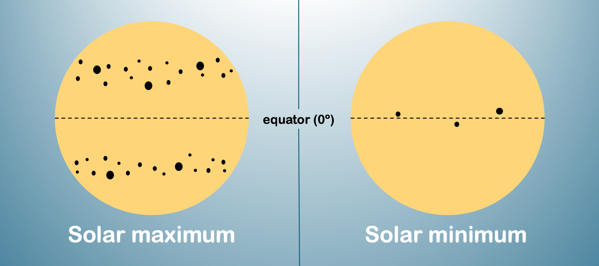
Figure 1: Schematic of sunspot latitude and frequency during a solar maximum and a solar minimum. [Annelia Anderson]
Besides telescopic observations, past solar activity can be estimated from the amount of carbon-14 in tree rings. Some of the carbon-14 in Earth’s atmosphere is created by cosmic rays interacting with atmospheric nitrogen. When the Sun is especially active, its enhanced magnetic field shields Earth from cosmic rays, which results in less carbon-14 in the atmosphere for trees to absorb. Results can be hard to interpret, though, because other factors like weather have a greater effect on carbon-14 production than solar activity does. Some carbon-14 solar cycle reconstructions have suggested extremely short solar cycles before the Maunder Minimum, while others have found solar cycles with regular to slightly long durations.
Understanding the onset of the Maunder Minimum is further complicated by the fact that telescopic sunspot observations only began in 1610 (just after the invention of telescopes). Observations began sometime during Solar Cycle −13, making it difficult to determine exactly when the cycle began — and therefore, difficult to determine whether the duration of Solar Cycle −13 was anomalous. Luckily for the authors of today’s article, a bit of data exists from the time before telescopes — drawings made by Johannes Kepler, the highly influential German astronomer best known for his laws of planetary motion, as he observed sunspots via camera obscura.
Kepler’s 1607 Sunspot Drawings
On 28 May 1607, Kepler made two sunspot drawings and recorded his activities and observations throughout the day. According to his book Phaenomenon singulare seu Mercurius in Sole (Kepler originally interpreted these sunspots as a transit of Mercury), his afternoon went like this:
Around 4:00 PM, Kepler noticed the clouds were clearing. There was a sunspot group large enough to be seen by the naked eye, so he headed home to observe the Sun. His house was on the bank of the Vltava River in Prague, and inside he had converted a room into a camera obscura — by only allowing the Sun’s light to enter through a pinhole, he was able to project an image of the Sun onto a sheet of paper. He traced this image and the large visible sunspot group. Next, he headed to the workshop of his friend Jost Bürgi, a Swiss clockmaker and mathematician. On his way there, he passed the Old City Hall, which had an astronomical clock that measured time since the previous sunset. The clock read 21 ⅓ hours. Once in Bürgi’s workshop, Kepler repeated his camera obscura observation, traced the Sun again, and noted that the Sun was setting when he finished. See Figure 2 for a depiction of his observations.
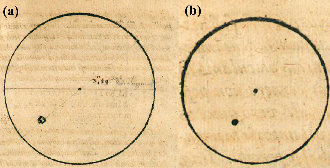
Figure 2: Kepler’s 28 May 1607 sunspot drawings. Left: Observation at Kepler’s house. Right: Observation at Bürgi’s workshop. [Adapted from Hayakawa et al. 2024]
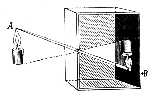
Figure 3: Diagram of a camera obscura. As the light travels through the pinhole, the projected image is inverted. [Fizyka z 1910 via Wikimedia Commons; Public Domain]
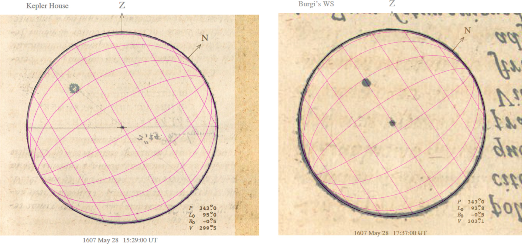
Figure 4: Kepler’s sunspot drawings overlaid with heliographic coordinates after reorientation. The Sun’s equator is the line that passes through the midpoint of each circle. Left: Observation at Kepler’s house. Right: Observation at Bürgi’s workshop. [Hayakawa et al. 2024]
Regular Solar Cycle Durations
Because many sunspots were visible at high latitudes in the years following 1610, the authors were able to place the beginning of Solar Cycle −13 (and end of Solar Cycle −14) somewhere between 1607 and 1610. Solar Cycle −13 ended around 1620, meaning it had a regular duration of 11–14 years. As an end date for Solar Cycle −14, these results also agree with carbon-14 solar cycle models in which Solar Cycle −14 lasts around 14 years.
In recent years, the Sun’s activity appeared to be decreasing and discussion arose around the possibility that we could be approaching another Maunder-like event. Though not a cause for concern, the possibility highlights the importance of studying and predicting changes in the Sun’s activity. Using Kepler’s pre-telescope drawings to show that previously contentious solar cycle durations were typical before the Maunder Minimum adds another piece to this unsolved puzzle.
Original astrobite edited by Caroline von Raesfeld.
About the author, Annelia Anderson:
I’m an astrophysics PhD student at the University of Alabama, using simulations to study the circumgalactic medium. Beyond research, I’m interested in historical astronomy and hope to someday write astronomy children’s books. Beyond astronomy, I enjoy making music, cooking, and my cat.


