bursts onto the Scene!")
Messier 82 (Star)bursts onto the Scene!
Editor’s Note: Astrobites is a graduate-student-run organization that digests astrophysical literature for undergraduate students. As part of the partnership between the AAS and astrobites, we occasionally repost astrobites content here at AAS Nova. We hope you enjoy this post from astrobites; the original can be viewed at astrobites.org.
Title: An In-Depth Study of Gamma Rays from the Starburst Galaxy M82 with VERITAS
Authors: The VERITAS Collaboration
Status: Published in ApJ
Starbursts: Not Just a Candy!
Cosmic rays are charged particles (electrons, protons, and atomic nuclei) that we’ve known about for more than a century. These particles notoriously zig and zag around the universe due to magnetic fields that attract them and then shoot them off in whichever direction the field goes. This makes it really hard to figure out what’s making them, especially because we detect them up to really high energies (petaelectronvolt-scale) — thousands of times more energetic than the particles accelerated at accelerators like the Large Hadron Collider! The mystery of what out there in the universe is making cosmic rays at these high energies has plagued astronomers ever since we discovered that cosmic rays exist in the first place.
Luckily, there are other ways to figure out where these enigmatic particles are made, including using plain old light — namely, gamma rays. Cosmic rays produce gamma rays in all sorts of different interactions with the material in the sources where they’re born. In other words, a cosmic-ray source should also be a gamma-ray source! By looking at how the gamma rays from a given astronomical object are distributed in brightness and energy (i.e., the spectral energy distribution), we can figure out what sort of cosmic rays make the gamma rays we observe and identify the big cosmic-ray factories of the universe.
Starburst galaxies (often just called “starbursts”), as their names imply, are galaxies that are forming stars very quickly — at rates 10–30 times higher than the Milky Way. This is probably just a phase, though, since these galaxies will quickly use up all their star-forming material (i.e., gas and dust) and will need to wait for this material to be re-released in supernovae or planetary nebulae when their stars eventually die.
We’ve long thought that starbursts might be cosmic-ray factories, as they host several high-energy processes such as supernovae and stellar winds launched by massive stars, hitting the dense material in star-forming regions. Since these processes don’t occur on anywhere near the same scales in our own Milky Way galaxy, we need to look elsewhere to understand if these processes are responsible for cosmic-ray production.
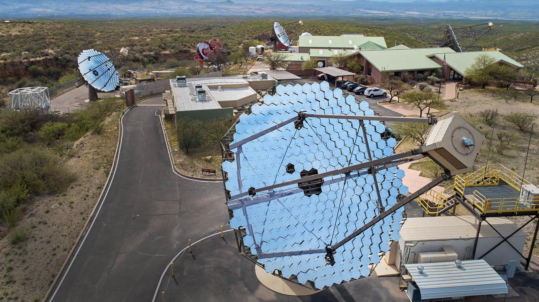
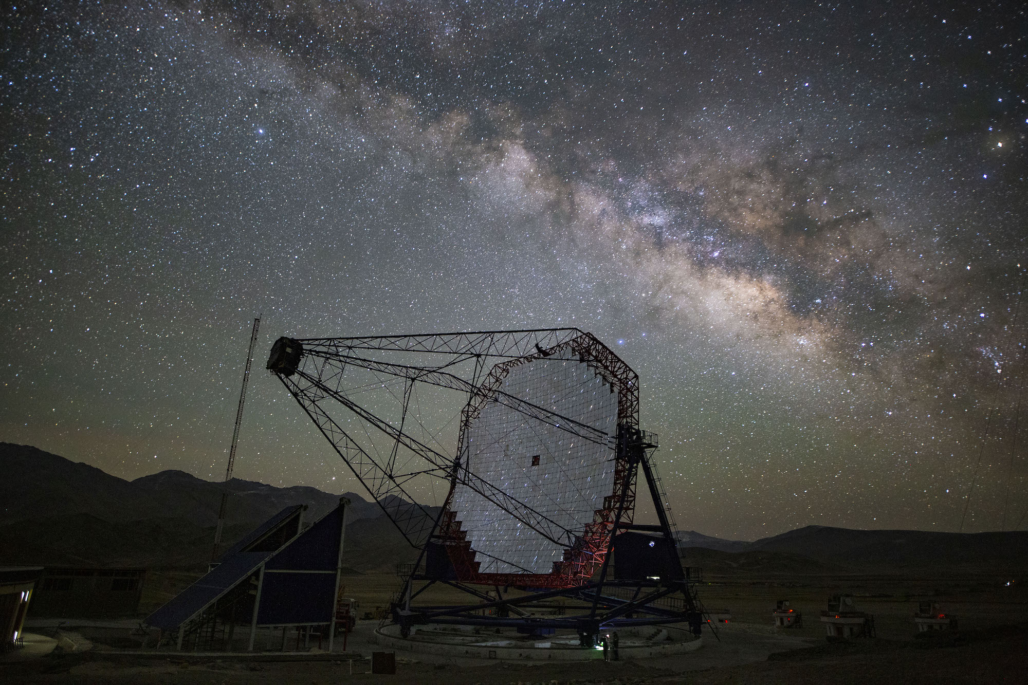
Figure 1: The VERITAS gamma-ray telescopes, which are located in southern Arizona, USA. [Center for Astrophysics | Harvard & Smithsonian]
Long Time, No Gammas
Today’s article follows up on a previous attempt to study M82 with VERITAS in 2009, which frustratingly resulted in the weakest detection VERITAS has ever reported — even after 137 hours of observations! More than a decade later, the VERITAS collaboration is back with a solid detection of gamma-ray emission from M82 (see Figure 2) and enough data to give M82 the attention it deserves!
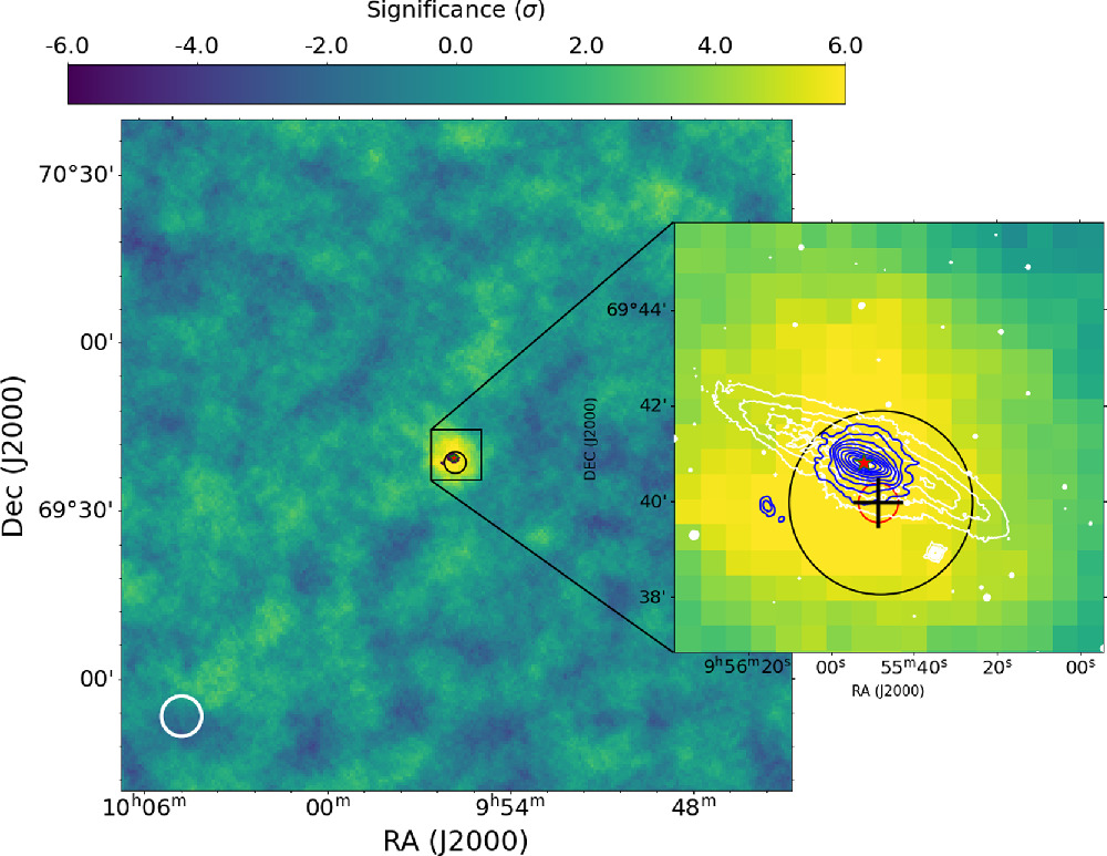
Figure 2: Sky map of the region surrounding M82, showing the statistical significance that the gamma rays observed aren’t just random background gamma rays or cosmic rays (higher significance is better!). The angular resolution of gamma-ray telescopes is not very good compared to other wavelengths. This can be seen in the inset, which shows the contours of optical data (white) and radio data (blue), with the best-fit and location of the VERITAS data denoted by the black circle and cross. The white circle in the bottom left shows VERITAS’s point spread function, which dictates the resolution of the image. [VERITAS Collaboration 2025]
It’s All in the Spectrum!
Even though M82 is 12 million light-years away (or more than a billion trillion kilometres), we can still learn an incredible amount of information about its subatomic particles, which are over half a million times smaller than a single human hair! The authors accomplish this by looking at the spectral energy distribution (see Figure 3), which shows how M82’s brightness changes with the energy (or frequency) of the gamma rays and any other light we observe.
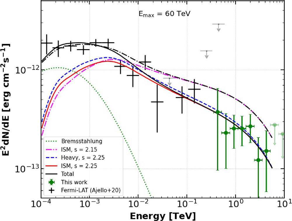
Figure 3: The leptonic and hadronic fits to the gamma-ray emission from M82, with Fermi-LAT data in black and VERITAS data in green. The leptonic (electron-only) model is shown by the green dashed line (called bremsstrahlung or braking radiation). The hadronic components are any of the pink, blue, or red lines, with each representing different average particle masses (denoted here with the particle’s rigidity, s, which is sort of a proxy for mass — or more precisely, how easily the particle is deviated by magnetic fields). They infer the types of particles from our own galaxy’s interstellar medium (ISM) and assume that M82 should be similar. All of these components are needed to find a fit to the data, as represented by the black solid line. [VERITAS Collaboration 2025]
What gets a little bit hairy is that hadronic particle interactions (protons/nuclei hitting things, accelerating, decaying, etc.) will also make a bunch of electrons called secondary electrons in the process, making it so that the authors are unlikely to see the proton/nuclei-only scenario. The spectrum is more likely to look more like a blend of both electrons and hadrons, even if electrons aren’t initially involved. These electrons are created after sudden bursts of star formation produce a bunch of cosmic rays, which will go on to make these secondary electrons that will stay within the galaxy over much longer timescales, leaving a lasting imprint of the cosmic-ray production that can be measured long after the star formation stops.
The authors compare leptonic (electron-only) and hadronic models to the observed gamma-ray data, to see which particles are responsible for making the gamma rays. They find that at least some hadronic component is needed to fit the observed gamma-ray data from the Fermi Large Area Telescope (Fermi-LAT) and VERITAS (see Figure 3), meaning that M82 is probably making cosmic rays that are protons and nuclei. They can also infer properties of the cosmic rays, such as the maximum energy of 60 teraelectronvolts, which is really impressive but doesn’t quite make it to the petaelectronvolt benchmark of the mystery cosmic-ray population (1,000 times the energy of M82’s particles). We know supernovae can get close to this benchmark, but we still don’t know what’s producing the higher-energy particles.
Star Light, Star Bright, Starburst!
Starbursts are promising sources that might be producing the elusive high-energy cosmic rays that astronomers have been hunting for more than a century. They also give us a larger sample size of star-powered sources that may allow us to gain more understanding about the smaller populations of supernova remnants and massive stars that exist in our own Milky Way. With the next-generation gamma-ray telescopes coming online soon (like the Cherenkov Telescope Array Observatory, which can detect gamma-ray sources in one-tenth the time it takes current-generation telescopes like VERITAS), hopefully studying these challenging and gamma-ray-dim sources will only be easier and more fruitful from this point forward!
Disclaimer: Today’s author was an author on this research article as a member of the VERITAS collaboration but was not directly involved in this project.
Original astrobite edited by Pranav Satheesh.
About the author, Samantha Wong:
I’m a graduate student at McGill University, where I study high energy astrophysics. This includes studying all sorts of extreme environments in the universe like active galactic nuclei, pulsars, and supernova remnants with the VERITAS gamma-ray telescope.
 Nothing to See")


 Breaks")