Ia’m Just Getting Started: A Type Ia Supernova’s First Day
Editor’s Note: Astrobites is a graduate-student-run organization that digests astrophysical literature for undergraduate students. As part of the partnership between the AAS and astrobites, we occasionally repost astrobites content here at AAS Nova. We hope you enjoy this post from astrobites; the original can be viewed at astrobites.org.
Title: The First Day of a Type Ia Supernova from a Double-Degenerate Binary
Authors: Gabriel Kumar, Logan J. Prust, and Lars Bildsten
First Author’s Institution: University of California, Santa Barbara
Status: Published in ApJ
Much like distance markers along the highway, Type Ia supernovae have long been used as distance indicators in space. These supernovae were originally theorized to form in binary systems. In this system, a white dwarf (a dense, collapsed remnant of a star) steals surface material from a non-degenerate star like our Sun and then explodes. Because of the initial conditions and properties of those two stars, the explosion would shine with the same intrinsic brightness regardless of the binary system’s location in space.
Research and observations, however, show that this is not entirely true; not all Type Ia supernovae are equally luminous. There are various theories regarding the different formation scenarios and explosion mechanisms that might create a Type Ia supernova. Developing ways to sleuth out the origins of these systems can be useful because it may tell us more about their luminosity.
One emerging theory of formation is the “double-detonation scenario.” In this case, two white dwarfs exist in a binary system. The more massive primary (the “accretor”) steals material from the less massive white dwarf secondary (the “donor”). After the primary steals the donor’s outer thin shell of helium, the helium surrounding the accretor detonates. This explosion induces a shock wave that travels into the dense core of the accretor and causes another detonation. The two detonations — one on the surface and one in the core — produce enough energy to explode the star into a supernova, a powerful stellar explosion. When the material from the exploding star reaches its companion star, it forms a mysterious, conical wake within the gaseous material, or “ejecta,” expelled from the accretor. This wake might be an important clue for distinguishing a supernova’s origins.
Since these explosions are incredibly powerful and would be difficult (and dangerous!) to perform in a lab, astronomers turn to computer simulations to model these events. Hydrodynamical simulations, in particular, are helpful for researchers because they model how fluids “flow” by solving complex equations that are too tricky to do by hand. (Remember that stars are just balls of gas, and hence fluid!) The authors of today’s article ran hydrodynamical simulations of the explosion and subsequent evolution of the ejecta from a double-detonation scenario.
In the diagram of the team’s setup (see Fig. 1), you can see a “bow shock.” This shock is from the wave produced in the accretor’s detonation and is bowed since it bends around the donor star. This shock moves quickly through the cone of ejecta, modifies its structure, and leaves clues within the ejecta as it settles.
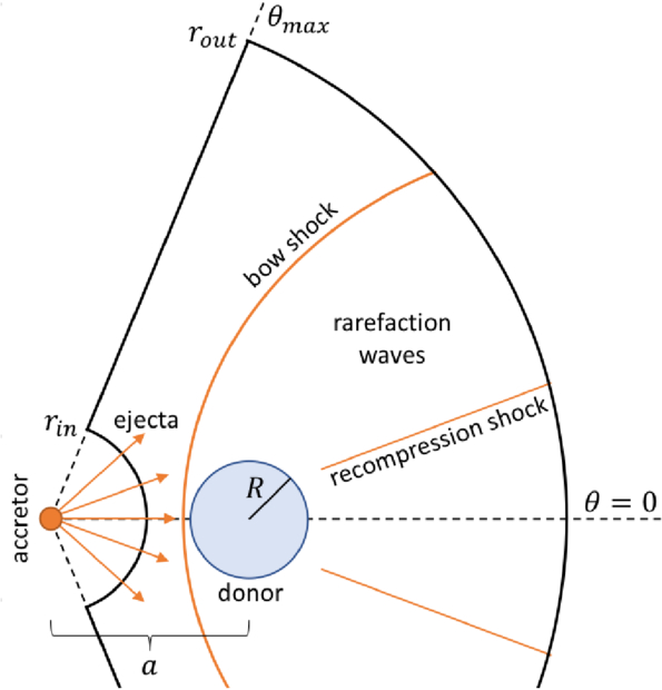
Figure 1: A visual schematic of the simulation setup. The accretor is the exploding star, which produces a “bow shock” from the detonation. The bow shock and recompression shock modify the structure of the ejecta, which fills the space between rout and rin. The ejecta is full of gaseous stellar material. [Kumar et al. 2025]
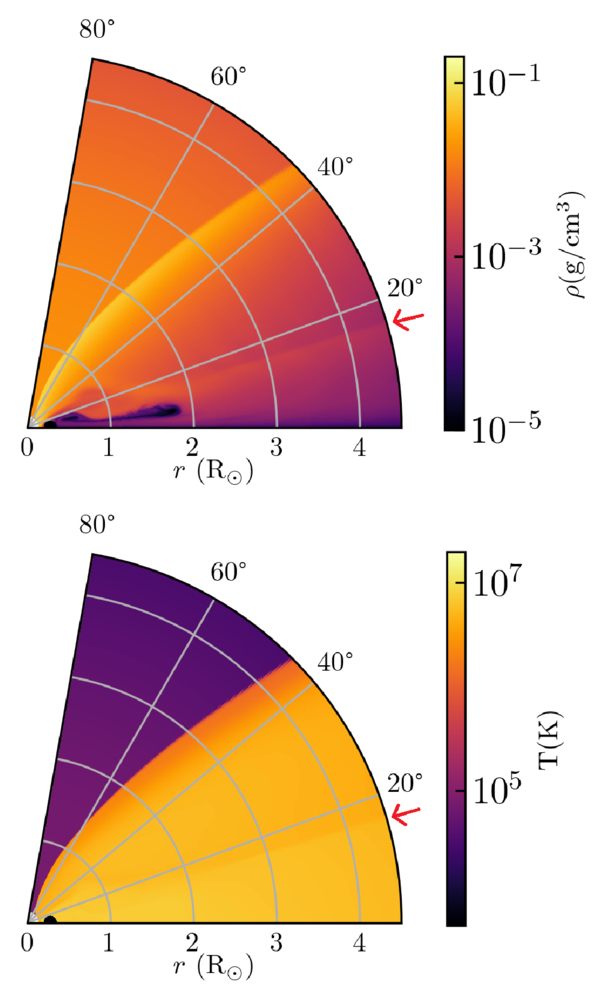
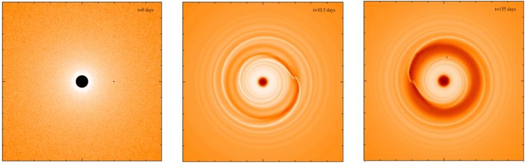
Figure 2: A visual “slice” of the ejecta surrounding the donor star just 200 seconds after detonation. The bottom-left corner (r = 0) has a faint white spot, indicating the donor. The density (top) and temperature (bottom) of the ejecta are shown. The faint line marked by the red arrow indicates the secondary shock from the explosion, highlighting changes in both density and pressure. [Kumar et al. 2025]

Figure 3: A slice of the simulation taken later, at 2 hours of simulation time. The ejecta in the shocked region has flown out farther than the ejecta in the unshocked region. Note that the horizontal scale has changed from Figure 2. [Kumar et al. 2025]
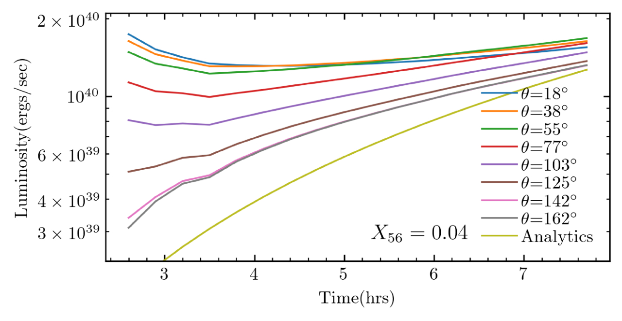
Figure 4: A comparison of luminosity vs. time over the course of 6 hours shortly after detonation. The different lines indicate different viewing angles from the axis of explosion. The line “Analytics” describes a light-curve prediction by Piro (2012) for a supernova that was not shock-heated. The luminosities for this model span almost one order of magnitude. [Kumar et al. 2025]
While there is always more work to be done, this work presents a first step at identifying double-detonation Type Ia supernovae from early observations. With an influx of observations from new observatories, like the Vera C. Rubin Observatory, we should expect to see many more early supernova detections.
Original astrobite edited by Ansh Gupta.
About the author, Mckenzie Ferrari:
I’m currently a PhD student in the geophysical sciences program at the University of Chicago. While I now study the atmosphere and oceans of Earth, most of my previous research focused on simulations of Type Ia supernovae and galaxy formation and evolution. In my free time, I foster cats for a local organization, enjoy cooking, and can often be found running along Lake Michigan.


 Too Hot to Handle?")