Feed the Fire, Fade the Metals
Editor’s Note: Astrobites is a graduate-student-run organization that digests astrophysical literature for undergraduate students. As part of the partnership between the AAS and astrobites, we occasionally repost astrobites content here at AAS Nova. We hope you enjoy this post from astrobites; the original can be viewed at astrobites.org.
Title: Metal-Poor Star-Forming Clumps in Cosmic Noon Galaxies: Evidence for Gas Inflow and Chemical Dilution Using JWST NIRISS
Authors: et al.
First Author’s Institution: Arizona State University
Status: Published in ApJ
If you want to reconstruct a galaxy’s life story, one of the best “fossil records” is its metallicity. In astronomy this refers to the abundance of elements heavier than helium, which are made in stars and returned to a galaxy’s gas through winds and supernovae. Over time, more star formation usually means more metals mixed into the gas.
Now zoom to Cosmic Noon (roughly when the universe was most actively forming stars). Many galaxies in this epoch look “clumpy”; their star formation is concentrated in several bright knots scattered across the disk. The big question is where those clumps come from. Do they form from the galaxy’s own gas via internal disk instabilities, or do they light up when fresh, metal-poor gas flows in and both fuels star formation and dilutes the local metallicity?
The authors try to answer that question with JWST by measuring the metallicity of each clump relative to its immediate surroundings, rather than comparing clumps to a single galaxy-wide number (which can be misleading if the galaxy has a metallicity gradient).
They use JWST/Near Infrared Imager and Slitless Spectrograph (NIRISS) slitless grism spectroscopy from the CAnadian NIRISS Unbiased Cluster Survey (CANUCS) to study 20 lensed galaxies at redshift 0.6 < z < 1.35. (Lensing effectively acts like a zoom lens, helping to resolve smaller structures.) They focus on emission lines that trace star-forming gas, especially Hα (a star formation tracer) and sulfur lines [SII] and [SIII] (needed for their metallicity method).
Slitless spectra come with a headache: because there is no slit, different parts of a galaxy can overlap in the dispersed image. To make reliable emission-line maps from slitless data, the authors use a forward-modeling code called Sleuth, which allows the continuum to vary across the galaxy.
The authors identify clumps using the Hα map together with rest-frame ultraviolet imaging because these tracers are sensitive to star formation on different timescales: Hα highlights gas ionized by the youngest massive stars, while ultraviolet light traces young stellar light over longer periods. As a result a clump can be bright in one and not the other, especially if dust is involved.
To estimate gas-phase metallicity, they use the “strong-line” method, which infers metallicity from ratios of bright emission lines calibrated using models and empirical samples. Their main diagnostic is S23 = ([SIII] + [SII]) / Hα. Because some line ratios also depend on the ionization state (how strongly the gas is being ionized by young stars), they also use the sulfur ratio S32 = [SIII]/[SII] as a check and iterate to a self-consistent solution.
So, Are Clumps Really Chemically Different from Their Surroundings?
For each clump, the authors measure the metallicity inside the clump and compare it to an annulus just outside the clump (masking neighboring clumps to avoid mixing). When they plot “clump metallicity” versus “local disk metallicity,” most points fall below the 1-to-1 line, meaning the clumps are more metal poor than their surroundings (Figure 1). The mean offset is about 0.1 dex, which corresponds to roughly 20% dilution in the clump gas.
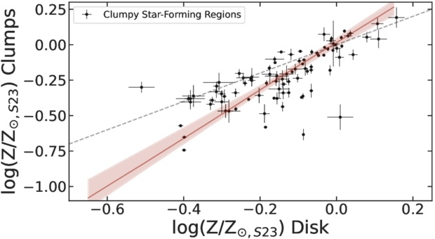
Figure 1: Each point compares a star-forming clump’s gas-phase metallicity to the metallicity of the nearby disk region immediately surrounding it. If clumps and disks had the same metallicity, they would lie on the dashed 1-to-1 line. Instead, most clumps sit below it, showing a typical ∼0.1 dex metallicity deficit, consistent with local chemical dilution. (The solid red line shows a best-fit linear trend to the clump measurement.) [Adapted from Estrada-Carpenter et al. 2025]
If inflow is really the driver, you should expect a link: the more strongly a clump is forming stars relative to its surroundings, the more diluted its metallicity should be. That is exactly what the authors find. The clumps that are most boosted in star formation are also the most metal diluted.
The article also emphasizes that clumps are not chemically uniform blobs. In at least one detailed example, the peaks in Hα (highest star formation) coincide with local minima in metallicity along a cut through the galaxy (Figure 2), suggesting internal star formation rate and metallicity gradients that reinforce the same story, intense star formation goes hand in hand with lower metallicity in the clump regions.
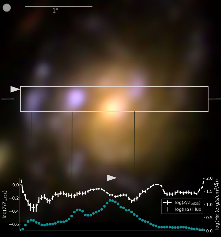
Figure 2: Example galaxy from this study illustrating the clump-scale link between star formation and metallicity. The color image shows the galaxy with a rectangular strip marking the region used for a 1D cut. In the bottom panel, the turquoise line shows the Hα flux (a tracer of recent star formation), while the white line shows the metallicity along the same cut. Peaks in Hα flux line up with local dips in metallicity, showing that the brightest star-forming clumps are also the most chemically diluted compared to nearby regions. [Adapted from Estrada-Carpenter et al. 2025]
Are These Clumps Really “In Situ,” or Could They Be Small Satellites?
A reasonable alternative is that some clumps are actually small companion galaxies projected onto the disk. These could also look metal poor, because low-mass galaxies tend to be low metallicity. The authors look for evidence using face-on systems and find that more massive clumps tend to sit closer to galaxy centers, which is consistent with in-situ clumps that form in the disk and migrate inward, though it does not rule out satellites. They argue that kinematics from JWST/NIRSpec IFU will be needed for a definitive separation.
Why This Matters
Gas inflow, star formation, and feedback, together known as the baryon cycle, are key drivers of how galaxies grow. What this article adds is a spatially resolved view that compares each clump to its local environment, showing that regions of elevated star formation also tend to be locally metal poor. That pairing is hard to explain as a simple metallicity gradient or a galaxy-wide averaging effect, and it is exactly what you would expect if at least some clumps are being fueled by relatively metal-poor inflows. In short, these clumps may be snapshots of galaxies refueling in real time.
Original astrobite edited by Ryan White.
About the author, Niloofar Sharei:
I’m an astronomy PhD candidate at UC Riverside studying how galaxies grow through star-forming clumps. I track how these clumps emerge, evolve, and sometimes survive long enough to reshape their galaxies. When I’m not thinking about cosmic blobs, I’m reading, hiking, or listening to Bach.