Astrobites RSS

high-redshift galaxy

Editor’s note: Astrobites is a graduate-student-run organization that digests astrophysical literature for undergraduate students. As part of the partnership between the AAS and astrobites, we occasionally repost astrobites content here at AAS Nova. We hope you enjoy this post from astrobites; the original can be viewed at astrobites.org.

Title: The MOSDEF survey: a stellar mass-SFR-metallicity relation exists at z∼2.3
Authors: Ryan L. Sanders et al.
First Author’s Institution: University of California, Davis
Status: Published in ApJ

Galaxy evolution is a complicated thing! Our current theory is that gas comes in, stars get made & explode, the surrounding interstellar medium (ISM) heats up and gets enriched with metals, and then gas goes out. These processes are happening in different stages all across the galaxy and can make simulating and observing galaxy evolution very difficult. Thankfully, through years of observation of local galaxies, we know that some galactic properties are correlated! For example, Tremonti et al. (2004) showed that there is a relation between stellar mass (M) and gas-phase oxygen abundance (12 + log(O/H) or Z) in the local universe (redshift z ~ 0). In 2008, Ellison et al. discovered that this M–Z relation also has a dependence on the star-formation rate (SFR), in the local universe. This local M–SFR–Z relation was shown later to be more correlated than the M–Z relation on its own!

The questions that then arise are: is there also evidence for a M–SFR–Z relation at high redshift? And if so, does it agree with the one at ~ 0? Or does it evolve with redshift? Many studies have tried to answer these questions, but most were based on large samples with low signal-to-noise (S/N) or small samples with intermediate S/N and have relied on a single metallicity indicator. But a 2018 study using a new, deep survey has changed that.

What Did They Do?

Completed in May 2016, the MOSFIRE Deep Evolution Field (MOSDEF) survey was a 4-year program in which the MOSFIRE instrument on the 10-m Keck 1 telescope was used to get near-IR spectra of ~1,500 galaxies spanning redshifts 1.4 < z < 3.8. The authors of today’s article elected to use the ~700 galaxies observed in the 2.01–2.61 redshift range. After S/N cuts, the authors were left with a 260-galaxy sample with an average redshift of z ~ 2.3 (see Figure 1, left). To make a conclusion about the (possible) redshift evolution of the M–SFR–Z relation, the authors used a comparison sample of 208,529 star-forming galaxies at ~ 0 from Andrews & Martini (2013).

redshift and star formation relations

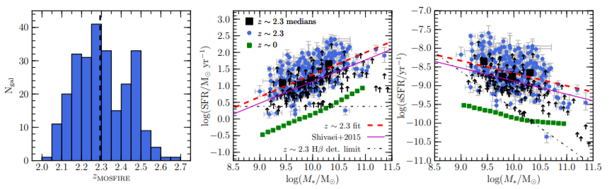
Figure 1: Left: The redshift distribution of their sample. The median redshift is z = 2.29. Middle: The SFR–M relation of the sample. Right: The sSFR–M relation of the sample. Here sSFR is the “specific star-formation rate,” which is just SFR/M. In the right two sections, the red-dashed line shows the best fit to the z ~ 2.3 data. This best-fit relation will be used when calculating the M–SFR–Z relation. [Sanders et al. 2018]

From their near-IR spectra, the authors measured SFRs from the H-alpha luminosities, which were then reddening-corrected. This correction is needed because dust grains between us and the galaxies scatter blue light and cause the galaxies to appear redder than they really are. Using broad- and mid-band photometric fits, the authors were able to robustly determine galaxy masses. Finally, using six emission-line ratios (which they abbreviate as N2, O3N2, N2O2, O3, R32, & O32; see the paper for definitions), they were able to get several metallicity estimates for each galaxy. Here, metallicity refers to the gas-phase oxygen abundance, 12 + log(O/H).

What Did They Find?

The authors did detect a M–SFR–Z relation at z ~ 2.3! This is best shown in Figure 2. This relation was found using the metallicity estimates from O3N2, N2, and N2O2. The ratios for R32 and O3 are double-valued with metallicity (think of these like a parabola) and can’t be used empirically to discover a relation like this. They can, however, be used to support a finding; in this case, the results from R32 and O3 are consistent with those found from the other three. Results from O32 were inconsistent with their findings and the authors concluded that this was likely due to biases in the reddening correction. Another main goal of this project was to determine if the M–SFR–Z relation evolved with redshift — and the authors found that it did! At a given mass and SFR, the metallicity of the z ~ 2.3 sample is 0.1 dex less than the z ~ 0 sample, also shown in Figure 2. The authors speculate that this evolution may be caused by an increase in the mass-loading factor from ~ 0 to ~ 2 and by a decrease in the metallicity of infalling gas at ~ 2.

metallicity–M* relations

Figure 2: Shown above are the Z–M relations using O3N2, N2, and N2O2. Points are colored by star formation. Squares represent the z ~ 0 data set while stars represent the z ~ 2.3 set. The red-dashed line shows the best fit to the z ~ 2.3 data. We see a M–SFR–Z relation at z ~ 2.3 and at fixed mass and SFR, the z ~ 2.3 set has 0.1 dex smaller metallicity than the z ~ 0 set. [Sanders et al. 2018]

What’s Left to Discover?

The authors established that a M–SFR–Z relation exists at z ~ 2.3 and that this relation evolves with redshift. The existence of this relation implies that our understanding of galaxy evolution is right… at least up to z ~ 2.3. The next step is to investigate this relation at higher redshifts, but that is no trivial task. As shown through the use of five emission-line ratios, measuring metallicities at high redshift can be difficult and will take great care. Uncertainties and inconsistencies with reddening corrections and other calibrations can cause large uncertainties in the results, like the case with O32. Thankfully, the introduction of large telescopes (like JWSTand TMT) will allow us to lessen these uncertainties through their increased sensitivities.

About the author, Huei Sears:

Huei Sears (she/her/hers) is a second-year graduate student at Ohio University studying astrophysics! Her research is focused on Gamma-Ray Burst host galaxies & how they fit into the mass-metallicity relationship. Previously she was at Michigan State University searching for the elusive period of B[e]supergiant, S18. In addition to research, she cares a lot about science communication, and is always looking for ways to make science more accessible. In her free time, she enjoys going to the gym, baking a new recipe, listening to Taylor Swift, watching the X-Files, and spending time with her little sister.

Koala

Editor’s note: Astrobites is a graduate-student-run organization that digests astrophysical literature for undergraduate students. As part of the partnership between the AAS and astrobites, we occasionally repost astrobites content here at AAS Nova. We hope you enjoy this post from astrobites; the original can be viewed at astrobites.org.

Title: The Koala: A Fast Blue Optical Transient with Luminous Radio Emission from a Starburst Dwarf Galaxy at z = 0.27
Authors: Anna Y. Q. Ho et al.
First Author’s Institution: California Institute of Technology
Status: Accepted to ApJ

Furry Animals and Relativistic Transients

Astrophysicists love clever titles, and in transient astronomy, we can get some fun ones! Transient sky surveys discover thousands of new explosions every year, with each one receiving a name based on when it was discovered. For example, in 2018, a peculiar transient called Astronomical Transient (AT) 2018cow was discovered and aptly deemed “the Cow” after the last letters of its International Astronomical Union (IAU) name. Coincidently, the Cow happened to be so unique that it received worldwide acclaim as one of the most exciting discoveries of 2018!

Following its discovery, the Cow became the prototypical transient in a new class of explosions called Fast Blue Optical Transients (FBOTs), whose name is reflective of their unique observational signatures. After detection, FBOTs rise to peak brightness in only a few days (i.e. fast!) and have extremely hot temperatures, which makes them appear bluer in color than typical supernova explosions. However, astrophysicists are still puzzled at how objects like the Cow are formed: a black hole shreds a white dwarf? Or maybe a massive star implodes to form an accreting black hole or magnetar? Either way, FBOTs present a fresh mystery that can only be solved by finding and studying similar events!

Innocuous Bear or Violent Explosion?

The authors of today’s paper present the discovery of a fuzzy new FBOT, ZTF18abvkwla, which was nicknamed the “Koala” after the last four letters of its official transient name. Furry animals keep making their way into astrophysics! Unlike Earth-based koalas, this transient creature is anything but docile: observations spanning the electromagnetic spectrum revealed that the Koala was a luminous event whose turbulent explosion resulted in high temperatures and rapid ejection of stellar material. The Koala was first observed by the Zwicky Transient Factory and is located in a distant dwarf galaxy with a high star formation rate of 7 solar masses per year. The large number of new stars in the Koala’s host galaxy may indicate that this FBOT came from the explosion of a young massive star rather than from an older star system containing a white dwarf.

Koala and Cow light curves

Figure 1: Optical light curve of the Koala (points) and prototypical FBOT, the “Cow” (lines). The remarkable evolution of the Koala shows that it rose and fell in luminosity in only 5 days, but it had an energy output similar to a normal supernova explosion! [Ho et al. 2020]

As shown in Figure 1, the authors demonstrate that the Koala’s luminosity evolution (i.e., light curve) is very similar to the Cow’s: rising to peak brightness in only a few days, very blue colors and a rapid decline in magnitude. Consequently, studying how FBOT light curves evolve in time is a powerful tool in uncovering the origin of these mysterious explosions. For instance, FBOTs rise and fade too quickly (day timescales) to be powered by radioactive decay of heavy elements, which is the mechanism invoked for most supernovae and occurs on about week timescales.

To produce both a luminous and rapidly evolving light curve like the Koala’s, the author’s discuss the possibility that the explosion was powered by the collision of outflowing material with gas in the local environment. However, this gas must also be quite opaque to radiation since the spectrum (Fig. 2) does not show hydrogen or helium emission lines that typically occur from an explosion interacting with material surrounding the progenitor star. Contrary to the comfortable climates of Australia’s native bear, the Koala’s spectrum revealed that it was an incredibly hot explosion that reached temperatures > 40,000 Kelvin!

Koala optical spectrum

Figure 2: Optical spectrum of the Koala with host galaxy emission lines marked in black. The spectrum indicates that the Koala had a temperature >40,000 Kelvin. [Ho et al. 2020]

The final piece of the puzzle discussed in today’s paper is the detection of luminous radio emission coming from the Koala. Shown in Figure 3, the Koala has one of the highest radio luminosities of any FBOT-like event (black stars), which is an important clue in deciphering the mechanisms behind the explosion. Similar to the Cow, the authors conclude that the Koala’s observed radio emission arose from an outflow of material moving at almost half the speed of light. That’s 100 million times faster than a koala running on Earth! This turbulent ejection of material in the Koala may be linked to the formation of a central engine like a black hole or rapidly rotating neutron star. Such a compact object could accrete material from an exploded star and violently expel semi-relativistic gas that would be visible as radio emission.

transient radio luminosities

Figure 3: Radio luminosities of different transients: FBOTs (black), gamma ray bursts (orange), relativistic/normal supernovae (red/blue) and tidal disruption events (purple). Another study on new FBOT CSS161010 was published soon after today’s paper. The Koala’s high radio luminosity suggests an accelerated outflow of material from a central compact object. [Ho et al. 2020]

While not your average woodland critter, the Koala has exposed how little we know about where FBOTs come from and the physics behind their energetic explosions. Unfortunately, understanding their complex origins will be difficult, as the authors conclude that the revised rate of FBOT discovery is almost 3 orders of magnitude less than that of typical supernovae. Nonetheless, new advancements in sky surveys will increase the number of new FBOTs and, with any luck, they will have more animal-themed names!

About the author, Wynn Jacobson-Galan:

Hi there! My name is Wynn (he, him, his) and I am an NSF Graduate Research Fellow at Northwestern University where I work with Prof. Raffaella Margutti on supernova progenitor systems and transient astronomy. I am fascinated by the final moments of stellar evolution before a star dies and becomes the violent supernova explosions we observe across the universe everyday. Consequently, as a researcher, I am both a stellar physician and a mortician: I use observational astronomy to wind back the cosmic clock in order to understand how certain stars were “living” right before their explosive “death.” Outside of research, I enjoy reading (specifically 20th century literature) and skateboarding. Also, if I’m not playing music (trumpet & saxophone), I am usually trying to find fun live music in Chicago.

Magnetic Orion

Editor’s note: Astrobites is a graduate-student-run organization that digests astrophysical literature for undergraduate students. As part of the partnership between the AAS and astrobites, we occasionally repost astrobites content here at AAS Nova. We hope you enjoy this post from astrobites; the original can be viewed at astrobites.org.

Title: HAWC+/SOFIA Multiwavelength Polarimetric Observations of OMC-1
Authors: David T. Chuss et al.
First Author’s Institution: Villanova University
Status: Published in ApJ

OMC-What?

The Orion Molecular Cloud 1 (OMC-1) is part of the Orion Nebula, and one of the most massive star-forming regions in the solar neighborhood. The gas and dust within OMC-1 act as a nursery for young stars, providing them with the necessary materials to develop. As such a close and large stellar nursery, OMC-1 is an easily accessible and important laboratory for studying the still-mysterious conditions that surround and encourage star formation. Today’s paper contributes to our understanding of star formation by determining OMC-1’s magnetic field and dust properties using polarimetry (more on this technique later!).

OMC-1 is a particularly interesting target for magnetic field and dust measurements because of the variation in structure across the cloud, which is shown in Figure 1. In front of OMC-1, there is an HII region ionized by a relatively young group of stars, the Trapezium cluster. The west side of OMC-1 hosts the Kleinman-Low (KL) Nebula and the Becklin-Neugebauer (BN) object. The KL Nebula is a clump of molecular gas and dust with a bunch of massive stars inside, of which the BN object is the brightest. In the infrared, the KL Nebula appears to be exploding because stellar winds from the massive stars heat up the surrounding gas. The southeast region of OMC-1 contains the Orion Bar, a photodissociation region that is cold, neutral, and creates the divide between HII and molecular gas. These features contribute to a complex magnetic field structure within OMC-1 that today’s authors map with polarimetry measurements.

OMC-1

Figure 1: The OMC-1 region, with overlaid magnetic field lines. Blue shows the KL Nebula and BN object, gray shows the HII region ionized by the Trapezium cluster, and purple shows the Orion bar. [NASA/SOFIA/D. Chuss et al. & ESO/M. McCaughrean et al.]

So What Is This Polarimetry I Speak Of?

We’ve all heard of polarized sunglasses, which block sunlight and reduce glare. Thinking of light as a wave, it travels in one direction and oscillates in the two planes perpendicular to that direction of travel. Polarized sunglasses block out one of these planes of vibration, and allow only half of the light to travel through the lenses.

Polarization measurements in astronomy work much the same way. For today’s paper, we are looking at the infrared light that is emitted from dust, but stars and other sources can emit polarized light too. For dust, the primary concepts of polarization remain the same as the case of blocking light with sunglasses. However, instead of blocking the light, dust actually emits light that has one plane of vibration brighter than the other from the start. To understand the reason behind this, assume that the dust has an egg shape. Because there is more surface area along the long axis of the egg than the short axis, we get more emission traveling in the direction of the long axis. This creates a net polarization of the signal: we get more infrared light in the direction that is parallel to the long axis of the dust. Lots of theories suggest that dust aligns its long axis perpendicular to the magnetic field, so by measuring the direction of the polarization, we can infer the direction of the magnetic field!

Flying High

Today’s authors used the HAWC+ instrument onboard NASA’s airborne observatory (the Stratospheric Observatory for Infrared Astronomy, or SOFIA)  to look at the infrared emission of the dust in OMC-1. They measured the total flux and polarization at four different wavelengths, and the results of their measurements can be seen in Figure 2. Interestingly, they found that at the smaller wavelengths (upper two panels), the magnetic field direction near the BN/KL objects, represented by the white star, is radically different than the surrounding region. The authors also discovered that the magnetic field direction in the Orion Bar differs significantly from elsewhere in OMC-1, and the magnetic field strength and dust temperature are highest near the BN/KL explosion location.

Polarimetry of OMC-1

Figure 2: Polarimetry measurements at 53, 89, 154, and 214 microns. The star symbol represents the location of the BN object, while the Orion Bar can be seen at the lower left. Colors represent total intensity, with red the highest and blue the lowest. Lines represent magnetic field direction. Click and zoom in to notice the change in the magnetic field with wavelength near the BN object! [Chuss et al. 2019]

Sweeping (Up the Dust) Conclusions

So why the change in magnetic field direction and strength across the OMC-1 region? The authors propose some interesting explanations. Remember how the KL nebula appears to be exploding from stellar winds? Well, it’s possible that this explosion has compressed the magnetic field opposite the material that it spits out, creating the distinctly different direction of the magnetic field that we see at shorter wavelengths. And the reason we don’t see the same compression at longer wavelengths? Longer wavelengths are emitted by the colder dust (Wein’s Law) that is likely to be outside of the explosion range! The authors also provide an explanation for the change in magnetic field direction that is present in the Orion Bar: the magnetic field of the bar may run parallel to its long side. When the vector of the magnetic field along the bar is added to the vector of the magnetic field in the surrounding region, it is likely to cancel itself out.

These insights on the magnetic field structure of OMC-1 demonstrate the power of polarimetry in astronomy, and the HAWC+ instrument on SOFIA will continue to make similar measurements more prevalent for molecular clouds. Because molecular clouds act as stellar nurseries, learning about their properties (like the direction and strength of their magnetic field) provides us with a better understanding of star formation processes.

About the author, Ashley Piccone:

I am a second year PhD student at the University of Wyoming, where I use polarimetry and spectroscopy to study the magnetic field and dust around bowshock nebulae. I love science communication and finding new ways to introduce people to astronomy and physics. In addition to stargazing at the clear Wyoming skies, I also enjoy backpacking, hiking, running and skiing.

Active Galactic Nucleus

Editor’s note: Astrobites is a graduate-student-run organization that digests astrophysical literature for undergraduate students. As part of the partnership between the AAS and astrobites, we occasionally repost astrobites content here at AAS Nova. We hope you enjoy this post from astrobites; the original can be viewed at astrobites.org.

Title: A Large Population of Obscured AGN in Disguise as Low Luminosity AGN in Chandra Deep Field South
Authors: Erini Lambrides et al.
First Author’s Institution: Johns Hopkins University
Status: Submitted to ApJ

Light emanating from within a host galaxy travels a huge distance to reach an observer. Along its path, the photons can encounter obstacles that change their wavelength or diminish the total intensity of the light. Depending on the host galaxy’s orientation relative to Earth, said emission could even be impeded by material contained within the galaxy. This can make the identification and classification of the photon’s source much harder. Models predict that there are a huge number of active galactic nuclei (AGN) growing behind dense screens of gas and dust that surround their host galaxies. Deep X-ray surveys are thought to produce the most complete and unbiased surveys of the AGN population, but we have yet to observationally confirm the high predicted fraction of these obscured AGN. Today’s paper re-evaluated such a deep X-ray survey containing a large sample of AGN in the Chandra Deep Field South (CDFS) and investigated whether the lower luminosity sources are, in fact, bright sources hidden behind larger amounts of obscuring material than previously thought.

AGN model

Figure 1: Standard model of an active galactic nucleus. [Urry & Padovani 1995]

The original study contains approximately 500 X-ray selected AGN in the CDFS at redshifts above z = 0.5. For each detection, the original study calculated an estimate of the column density — a quantity describing the likely density of gas and dust around the galaxy that impedes photons travelling between the source and the observer. Using the column density of each AGN, today’s authors corrected the original observations and estimated an intrinsic X-ray luminosity. Assuming the original study calculated the column density correctly then this intrinsic X-ray luminosity should make all the AGN in the sample appear completely un-obscured. Alongside this, they gathered mid-IR (6 and 24 µm) and optical emission line data, which can be used to describe other aspects of the AGN’s behaviour.

Tales of the Un-Obscured

In an AGN, the observed X-ray emission is absorbed by material in the surrounding torus (Figure 1). This is then re-emitted at the 6 µm, mid-IR, wavelength by the torus. Assuming the original study correctly calculated the column density, we would expect these AGN to show a direct correlation between X-ray and mid-IR luminosity. However, there are a large number of AGN that have a much lower intrinsic X-ray luminosity for their torus luminosity, known as a ‘mid-IR excess’. In addition, 90% of these AGN are found in the faintest group of observations. Whilst this suggests that these faint AGN could be heavily obscured, there are a number of other possible explanations for why lower luminosity AGN have a mid-IR excess.

AGN luminosities

Figure 2: Comparing the intrinsic X-ray luminosity of an AGN against its torus luminosity. All of the AGN are coloured based on the group their observed flux falls into, with the faintest being blue ranging up to the most luminous in red. The dashed blue line highlights the region we expect an un-obscured AGN to lie within. [Lambrides et al. 2020]

One possibility is simply that the intrinsic X-ray luminosity is correct and we are observing an un-obscured AGN with genuinely lower emission than expected. In Figure 3, the authors compare the intrinsic luminosity to the [OIII] optical emission line luminosity — an independent measure of AGN activity — to see whether these AGN are intrinsically faint. Not only do the faint AGN (blue points) sit outside the region that suggests they are un-obscured, but they appear to be much more active than expected for their intrinsic X-ray luminosity and also occupy a similar region to obscured AGN from a previous study. So, these faint AGN don’t have an intrinsically lower activity, but they do behave similarly to obscured AGN.

AGN luminosity vs [OIII]

Figure 3: Comparing the intrinsic X-ray luminosity with the luminosity of the [OIII] optical emission line — an independent measure of AGN power. As with Figure 2, the AGN are coloured by their observed X-ray flux and we expect un-obscured AGN to lie within the dashed blue lines. There are also a number of AGN from a separate study: filled, grey points are un-obscured AGN and the hollow, grey points are obscured AGN. [Lambrides et al. 2020]

If the AGN aren’t less active then perhaps a non-AGN emission component, such as star formation, could be causing the mid-IR excess. 24 µm emission is commonly used to trace star formation as warm dust associated with high-mass star-forming regions emits strongly at this wavelength. However, 24 µm emission can also be associated with activity from un-obscured AGN. Figure 4 shows that whilst many of these AGN don’t sit within the un-obscured region, crucially none of them are anywhere near the star-formation-driven relationship. In particular, the faint AGN (highlighted with a red circle) occupy this in-between area where they don’t appear to behave like un-obscured AGN, nor are they all explained by star formation.

Intrinsic X-ray luminosity vs 24 µm luminosity

Figure 4: Comparing the intrinsic X-ray luminosity against the 24 µm luminosity. All of the AGN are coloured based on their redshift (as this determined the instrument recording 24 µm emission) but the lowest flux AGN (previously blue in Figures 2 & 3) are highlighted with red circles. Objects with 24 µm emission largely driven by the AGN are found in the grey region, whilst those driven by star formation would be found within the red region. [Lambrides et al. 2020]

Given that this mid-IR excess cannot be explained by a less active AGN or star-formation, the authors turn to their initial hypothesis: these faint AGN are more heavily obscured than the original study proposed. In Figure 5 the authors investigated how different levels of obscuration could help describe the observations. Most of the faint AGN (blue points) are consistent with column densities at least 10 times larger than calculated in the original study. Such an increase in obscuration would see a similarly sized increase in intrinsic X-ray luminosity and account for the mid-IR excess. Thus, the authors conclude that they have discovered a new sample of highly obscured AGN.

observed X-ray luminosity vs. torus luminosity

Figure 5: Similar to Figure 2, but instead comparing the observed X-ray luminosity with the torus luminosity. Overlain on these points are regions within which we would expect to find AGN of varying levels of obscuration. Un-obscured AGN are found within the red region, more heavily obscured AGN are found within the blue region. [Lambrides et al. 2020]

Today’s paper is important as it provides a new successful approach to probing a fainter luminosity population than previously investigated in the field. In addition, assuming that all the newly identified obscured AGN have an increased column density, then the authors find that estimations of the space density of obscured AGN increases between 40% – 50%, depending on redshift. Such an increase helps close gap between the observed and predicted densities of obscured AGN in the universe.

About the author, Keir Birchall:

Keir is a PhD student studying methods to identify AGN in various populations of galaxies to see what affects their incidence. When not doing science, he can be found behind the lens of a film camera or listening to the strangest music possible.

Planet 9

Editor’s note: Astrobites is a graduate-student-run organization that digests astrophysical literature for undergraduate students. As part of the partnership between the AAS and astrobites, we occasionally repost astrobites content here at AAS Nova. We hope you enjoy this post from astrobites; the original can be viewed at astrobites.org.

Title: Testing the Isotropy of the Dark Energy Survey’s Extreme Trans-Neptunian Objects
Authors: Pedro H. Bernardinelli, Gary M. Berstein, Masao Sako et. al
First Author’s Institution: University of Pennsylvania
Status: Submitted to The Planetary Science Journal (PSJ)

Out beyond the orbit of Neptune lie small solar system bodies called trans-Neptunian Objects (TNOs). They are rocky, icy, dirt balls that lie far beyond Neptune for the majority of their orbits, but their perihelia exist within the orbit of Neptune, or less than about 30 AU.

TNO orbits

Figure 1: The orbits of the seven trans-Neptunian objects discovered in the Dark Energy Survey. These are polar plots, so it’s similar to what we would see if we looked at the orbits of these objects from a (space)bird’s-eye view. The figure on the left shows the full extent of their orbits; green orbits have an aphelion (their furthest extent) greater than 250 AU, purple orbits have an aphelion between 150 and 250 AU. The dashed lines have a perihelion (closest approach to the Sun) less than 37 AU (so they get pretty close to Neptune), and the solid lines have a perihelion greater than 37 AU (so they are not strongly affected by Neptune’s gravity). The figure on the right is a zoom-in showing their perihelia compared to Neptune’s orbit in blue. [Bernardinelli et al. 2020]

Finding Anti-Symmetric Orbits

This paper uses data from the Dark Energy Survey (DES), which, while on the quest for dark energy signatures far beyond our solar system, has found some extreme trans-Neptunian objects (eTNOs, basically very distant TNOs). Based on the observed TNOs from DES, we can see that their orbits appear to be aligned. As you can see in Figure 1, they appear to lie on one side of the sky, having similar ecliptic longitudes. That’s weird, because things in space tend to be symmetrically distributed, or isotropic. So, shortly after astronomers saw these weirdly aligned orbits, an interesting hypothesis came about. Maybe there is a super-Earth located way beyond the orbit of Neptune that is pushing these TNOs onto these aligned orbits. That hypothesized planet was nicknamed Planet 9 and is still being hunted for after about 4 years of searching.

But What If We Just Aren’t Looking Hard Enough?

Before we hype up this underdog of a planet, we must ask ourselves, is Planet 9 really the most likely explanation for the TNO clustering? We have not observed the full TNO population. What if that population is actually isotropic, and we are just looking at a few members of that population that happen to be on one side of the sky? This is the question that today’s paper poses. Given how we observed these objects, and where we’ve pointed our telescopes, could the observed TNOs be just one part of an isotropic population? If so, then Planet 9 doesn’t need to exist.

This paper starts to explore that question by creating a simulated population of 40 million TNOs that are defined by certain orbital parameters. The longitude of the ascending node (ᘯ), argument of perihelion (⍵), and mean anomaly (M, which is approximately the angular distance of object from its pericenter), are all given random values, i.e., they are distributed isotropically, so there is no preferred value. The eccentricity, inclination, and aphelion are kept within certain values taken from the seven observed TNOs from the Dark Energy Survey.

orbital parameter schematic

Figure 2: Schematic showing the different orbital parameters used to characterize TNOs in this study. This study created a simulated population of TNOs that had ᘯ, ⍵, and the mean anomaly distributed randomly, but kept orbital parameters such as inclination, eccentricity, and aphelion consistent with observed TNOs. [Arpad Horvath]

They then look to pare down their simulated population to only include eTNOs that could have been observed with DES. That includes finding the eTNOs that are bright enough, have traveled a significant distance across the sky, and could have been seen for multiple days. If a TNO passes all of those tests, then it is deemed to be observable. This observable population is their final sample, with which they can then run some statistical tests. They want to compare the orbital parameters of this simulated sample to the TNOs that we have observed.

histograms of orbital parameters

Figure 3: Histograms showing the highest likelihood values for three orbital parameters that describe TNOs. There were four different eTNO cases explored based on differing definitions of what an eTNO is. The green and purple lines are the eTNOs that the Dark Energy Survey has discovered. [Bernardinelli et al. 2020]

This study ran two statistical tests to compare the two samples: Kuiper’s test and a likelihood test. From Kuiper’s test, they calculate a p-value; a higher p-value means that the two populations are similar. They run the test to compare the ᘯ,  ⍵, and ᘯ + ⍵ values found in the simulated population to that which was observed. In the likelihood test, they compare the observed orbital angles for each sample to produce an f-value, which can be converted to a % likelihood. A low percent means that it is very unlikely that the observed sample comes from an isotropic population and a high percent means that it is very likely.

They also had four different observed samples, each of which is a subset of the 7 observed eTNOs, and each case was motivated by a different definition what an eTNO is. Each case appears to be aligned to some degree. Case 1 – 4 went from lenient definitions to strict definitions describing eTNOs. Case 1 included all seven TNO objects, while Case 4 only included those that had an aphelion beyond 250 AU and a perihelion greater than 37 AU — which includes only three objects that appear to be strongly aligned. The most extreme TNOs are going to be least affected by Neptune, and most affected by Planet 9, if it exists.

They then ran their statistical tests on these four cases. They found that when they include all seven eTNOs, it agrees well with coming from an isotropic population — which means that Planet 9 is not necessary to explain the TNO orbits. When they go down to the most strict definition of eTNOs, the p-values tend to drop. This means it becomes less likely the eTNOs that we see come from an isotropic population, however the p-values are not low enough to completely rule that out.

So Are the Authors Trying To Kill Planet 9?

In the end, this paper was able to recreate the orbits of known TNOs using an isotropically distributed TNO population. This means that Planet 9 doesn’t need to exist. However, their results change when they run the same statistical test against 3 out of the 7 TNOs. In this case, it’s harder to show that these orbits come from a randomly distributed population, leaving some hope for the Planet 9 enthusiasts. When working with such a small sample size (seven objects!) it’s hard to come to a confident conclusion. The authors look forward to more years of DES so that more eTNOs can be discovered, improving our understanding of TNOs and the mysterious Planet 9.

About the author, Jenny Calahan:

Hi! I am a second year graduate student at the University of Michigan. I study protoplanetary disk environments and astrochemistry, which set the stage for planet formation. Outside of astronomy, I love to sing (I’m a soprano I), I enjoy crafting, and I love to travel and explore new places. Check out my website: https://sites.google.com/umich.edu/jcalahan

TDE

Editor’s note: Astrobites is a graduate-student-run organization that digests astrophysical literature for undergraduate students. As part of the partnership between the AAS and astrobites, we occasionally repost astrobites content here at AAS Nova. We hope you enjoy this post from astrobites; the original can be viewed at astrobites.org.

Title: Prompt Accretion Disk Formation in an X-Ray Faint Tidal Disruption Event
Authors: Tiara Hung et al.
First Author’s Institution: University of California, Santa Cruz
Status: Submitted to ApJ

To Catch an Accretion Disk

The universe reveals a variety of ways in which stars can die. We observe stars imploding, erupting, and merging, yet the tidal disruption event (TDE) is one of the most tumultuous spectacles of stellar destruction we have discovered so far. This transient phenomenon begins with a star orbiting near a supermassive black hole (SMBH) in the galaxy center. Oblivious to its impending doom, the star’s trajectory pushes it too close to the SMBH’s sphere of gravitational influence and tidal forces begin to shred the stellar structure. The woeful star is now a fly in a supermassive spider’s web: the star will be ripped apart, spaghettified stellar gas coming to form an accretion disk. This then results in a violent eruption of radiation as bits of star fall into the central black hole (Figure 1).

TDE H-alpha

Figure 1: Artist’s interpretation of a tidal disruption event (TDE). Here a star is shredded by a supermassive black hole, forming an accretion disk that then emits bright optical radiation. The type of hydrogen emission from a TDE is dependent on whether we observe accretion disk (A) face-on or (B) edge-on. [Adapted from NASA/CXC/M. Weiss]

While we’ve detected nearly a hundred TDEs, the nature of how the star is disrupted and comes to form an accretion disk around a SMBH is still very much an open question. Theoretical predictions spanning the past two decades suggest that this infall of gas from the disrupted star can, however, be uniquely recognized in spectroscopic observations. For example, as shown in Figure 1 (A), a smoking-gun indication of accreting material would be to spot a double-peaked H-alpha emission line that arises from excited hydrogen being consumed by the SMBH. And now this exact signature was observed!

Theoretical Predictions Confirmed

In an exciting leap for the study of TDEs, the authors of today’s paper present the first confident detection of a newly formed accretion disk around a SMBH. The discovered explosion is a TDE called Astronomical Transient (AT) 2018hyz, which was observed spectroscopically by the team for over 300 days after the explosion was detected. In Figure 2 we see that by Day 51 the SMBH’s stellar consumption has revealed itself in the form of “horned” hydrogen emission line profiles.

TDE 2018hyz spectroscopy

Figure 2: Spectroscopic observations of TDE 2018hyz for over 300 days after the explosion was detected. By Day 51, we can see the infamous double-peaked line profiles emerge in H-alpha (marked in grey). These are directly linked with an SMBH accreting material from a disrupted star. [Hung et al. 2020]

This exquisite display of accretion around a SMBH allowed the authors to precisely model the TDE’s physical parameters such as the velocity, orientation, inclination, and eccentricity of the stellar gas being accreted. By running a 10-parameter grid search, the authors fit the peaked H-alpha emission in AT 2018hyz’s spectra with a multi-component model shown in Figure 3. Specifically, their modeling revealed that TDE 2018hyz was observed at a large enough inclination angle to allow for the detection of this double-peaked line profile, a direct signature of a visible accretion disk. The confirmation that TDE spectra are influenced by the angle at which we view the accretion disk will be extremely applicable to future TDE observations. This discovery has demonstrated that any TDE without double-peaked features was most likely observed with only the edge of the accretion disk visible to us.

model fits to TDE

Figure 3: Combined, multi-component model of the TDE shown in red. The dashed blue/green lines arise from the accretion disk while the dotted orange line is from the outward ejection of material after the star is ripped apart. [Hung et al. 2020]

The most exciting thing about confidently detecting an accretion disk is that it is now possible to distinguish between individual components of the TDE as a whole. For example, an accretion disk model cannot completely fit the H-alpha profile in Figure 3. The authors show that you also need a Gaussian line profile that physically represents a turbulent outflow of gas following the disruption of the star. While subtle, this newfound ability to separate the pieces of star plummeting into a SMBH from the gas that is violently ejected outwards will be instrumental in painting an accurate picture of how these brilliant bursts of radiation occur.

It should be noted that other teams have published journal articles on this same TDE, e.g., Short et al. 2020 and Gomez et al. 2020.

About the author, Wynn Jacobson-Galan:

Hi there! My name is Wynn (he, him, his) and I am an NSF Graduate Research Fellow at Northwestern University where I work with Prof. Raffaella Margutti on supernova progenitor systems and transient astronomy. I am fascinated by the final moments of stellar evolution before a star dies and becomes the violent supernova explosions we observe across the universe everyday. Consequently, as a researcher, I am both a stellar physician and a mortician: I use observational astronomy to wind back the cosmic clock in order to understand how certain stars were “living” right before their explosive “death.” Outside of research, I enjoy reading (specifically 20th century literature) and skateboarding. Also, if I’m not playing music (trumpet & saxophone), I am usually trying to find fun live music in Chicago.

illustris simulation

Editor’s note: Astrobites is a graduate-student-run organization that digests astrophysical literature for undergraduate students. As part of the partnership between the AAS and astrobites, we occasionally repost astrobites content here at AAS Nova. We hope you enjoy this post from astrobites; the original can be viewed at astrobites.org.

Title: MOSEL Survey: Tracking the Growth of Massive Galaxies at 2 < z < 4 using Kinematics and the IllustrisTNG Simulation
Authors: Anshu Gupta et al.
First Author’s Institution: University of New South Wales, Australia
Status: Published in ApJ

How, exactly, galaxies form is still very much an open question in astrophysics. It’s not like we can watch a galaxy evolve — most are about 12 billion years old, and even the youngest we’ve discovered is about 500,000 million years old.

There are two ways to work around this problem. The first is a simple matter of looking back into time. Light takes a finite amount of time to travel to us, and so the farther away we look, the older that light is. That means that the farther a galaxy is, the younger we see it. Instead of watching a single galaxy evolve over time, we can compare farther (“younger”) galaxies to closer (“older”) galaxies, and interpolate what may have happened to cause any changes.

The second way to work around our observational conundrum is to watch galaxies evolve in simulation space. The authors of today’s paper used IllustrisTNG100, part of a suite of large cosmological simulations of galaxy evolution. The cover image above shows a subset of luminous matter in the TNG100 simulation.

Observed Mass, Movement and Star Formation History

The kinematic properties (how things are moving) of star-forming galaxies is strongly linked to how they gained their mass. Today’s authors compared the velocity dispersion of observed “younger” galaxies at redshift z = 3.0–3.8 to “older” galaxies from previous studies of redshift ~ 2 and found that their most massive galaxies had smaller velocity dispersions than massive “older” galaxies.

velocity dispersion

Figure 1: Velocity dispersion as a function of mass, shown on a log–log scale. The authors’ “younger” galaxies are shown as gold stars. Other shapes represent previous studies of “older” galaxies at z ~ 2. The more massive galaxies in the authors’ sample are represented by larger stars and have smaller velocity dispersions than “older” galaxies of the same mass (shown in the red circle). [Adapted from Gupta et al. 2020]

By looking at the spectra of these galaxies, the authors could also extract their star formation histories. Basically, this looks at how old current stars are to extract the star formation rate over time. The top panels of Figure 2 show the authors’ results (keep in mind, time reads as newer on the left and older on the right). The bottom two panels show results from previous studies of galaxies at ~ 2. While the less massive galaxies in the authors’ survey (top left panel) show the same pattern of increasing star formation rate, the most massive galaxies on the right have relatively flat star formation histories. This is in contrast to massive galaxies at ~ 2, which show an increasing star formation rate over time.

star formation histories

Figure 2: Star formation histories for four different populations of galaxies. The x-axis is galaxy time before observation and the y-axis is star formation rate. The top two panels are the galaxies from the authors’ survey at z ~ 3 and the bottom two are from a previous survey at z ~ 2. The less massive galaxies are on the left and the more massive galaxies are on the right. The shaded areas indicate errors and the red arrows point toward trends. [Gupta et al. 2020]

Both the odd star formation histories and velocity dispersions point to something happening between = 3 and = 2 that changed massive galaxies. To determine what that might be, the authors turn to simulations.

Into the Simulation

The IllustrisTNG100 simulation starts with a distribution of mass at a redshift of = 127 and runs until present day, = 0. As it runs, the random fluctuations in density at = 127 turn into galaxies, which grow, form stars and merge. The authors wanted to look at how these galaxies acquired their stars over time.

There are basically two ways that a galaxy can gain stars: either by forming them from gas belonging to the galaxy (in situ) or by accreting the stars from other, mostly smaller, galaxies (ex situ). Figure 3 shows the fraction of stellar mass in the simulation that was accreted ex situ, rather than formed in the galaxy. It shows that for the most massive galaxies (in red), the fraction of ex situ stellar mass increases between = 3 (pink dotted line) and = 2 (black dotted line). Meanwhile, the ex situ stellar mass fraction remained largely constant for less massive galaxies (blue).

ex situ stellar mass fraction

Figure 3: The fraction of a galaxy’s stellar mass that was obtained from other galaxies, rather than formed in situ. Massive galaxies are shown in red, while less massive galaxies are shown in blue. The salmon and blue shaded regions are, respectively the error for the more massive and least massive galaxies. The black and pink dotted lines indicate, respectively, z = 2 and z = 3. [Gupta et al. 2020]

Uniting Simulations and Observations

The authors speculate that this increase in ex situ stellar mass fraction seen in simulations may be responsible for the increase in velocity dispersion seen in observed massive galaxies between = 3 and = 2. Turbulence and gravitational instabilities driven by accretion of stars and gas would increase the randomness of velocities (i.e. the velocity dispersion).

This could also explain the difference in star formation history between massive galaxies at = 2 and = 3 (Figure 2). Gas is necessary for the formation of stars and if the galaxies at = 2 have been able to gain gas from accretion, they would be able to increase their star formation rate, as seen in the bottom right panel of Figure 2. In contrast, a smaller ex situ stellar mass fraction for = 3 galaxies indicates that there has been less accretion and less opportunity to gain new gas and thus form new stars, leading to the flat star formation trend seen in the top right panel of Figure 2.

Essentially, the younger galaxies at = 3 have had less time to merge with other galaxies, leading to smaller velocity dispersions and less star formation.

The authors note that their conclusions are limited by many factors, including a small sample size. However, these are promising results and show how much can be gained by comparing observations and simulations.

About the author, Bryanne McDonough:

Graduate student at Boston University where I am currently studying the distribution of dark matter and satellites around galaxies using data from the Illustris simulations. My primary research interests are galactic and extragalactic astrophysics using computational methods. Outside of grad school I enjoy reading and crafting.

FRB

Editor’s note: Astrobites is a graduate-student-run organization that digests astrophysical literature for undergraduate students. As part of the partnership between the AAS and astrobites, we occasionally repost astrobites content here at AAS Nova. We hope you enjoy this post from astrobites; the original can be viewed at astrobites.org.

Title: Spectropolarimetric analysis of FRB 181112 at microsecond resolution: Implications for Fast Radio Burst emission mechanism
Authors: Hyerin Cho et al.
First Author’s Institution: Gwangju Institute of Science and Technology, Korea
Status: Published in ApJL

Fast radio bursts (FRBs) are probably the fastest growing and most interesting field in radio astronomy right now. These extragalactic, incredibly energetic bursts last just a few milliseconds and come in two flavors, singular and repeating. Recently the number of known FRBs has exploded, as the ​Canadian Hydrogen Intensity Mapping Experiment (CHIME) radio telescope has discovered about 20 repeating FRBs (and also redetected the famous FRB 121102) and over 700 single bursts (hinted at here). However, despite the huge growth in the known FRB population, we still don’t know what the source(s) of these bursts is (are). Today’s paper looks at possible explanations for the properties of one FRB in particular to try to figure out what its source might be.

Your Friendly Neighborhood FRB

A number of previous astrobites have discussed the basics of FRBs (here, here, and here for example) but the FRB that the authors of this paper focus on is FRB 181112. FRB 181112 was found with the Australian Square Kilometer Array Pathfinder (ASKAP) and localized to a host galaxy about 2.7 Gpc away from us even though it has not been observed to repeat. That’s over a hundred times farther away than the closest galaxy cluster, the Virgo Cluster! One quality of FRB 181112 that makes it particularly interesting to study is that the way ASKAP records data allows the authors to study the polarization of the radio emission. Polarization of light is a measure of how much the electromagnetic wave (here the radio emission) rotates due to any magnetic fields it propagates through. The two types of polarization are linear polarization (Q for vertical/horizontal, or V for ±45°), which occurs if the electromagnetic wave rotates in a plane, and circular (either left- or right-handed depending on the rotation direction) if the light rotates on a circular path. By looking at the polarization of FRB 181112, shown in Figure 1, the authors can determine the strength of the magnetic field it traveled through.

polarization profile

Figure 1: a) The full polarization profile of FRB 181112 showing four profile components. The black line, I, is the sum of all the polarizations of light, or the total intensity of the burst. The red line, Q, is the profile using only (linearly) horizontally or vertically polarized light; the green line, U, is using only the (linearly) ±45° polarized light; and the blue line, V, is the profile using only circularly polarized light. Negative values describe the direction of the polarization. b) The polarization position angle of the zoomed in profiles from panel (a) seen in panel (c). Variation here suggests the emission is coming from different places in the source. d) A three second time series of the data where the FRB is clearly visible at about 1.8 seconds. [Cho et al. 2020]

In addition to polarization, the dispersion measure (DM), or difference in time of arrival of the FRB at the telescope between the highest and lowest radio emission frequencies due to its journey through the interstellar medium (ISM), can provide information about the properties of the environment(s) the burst travels through. Each of the four components of FRB 181112 (visible in panel (a) of Figure 1 in three different polarizations, Q, U, and V, as well as total intensity, I) are shown in the bottom row of Figure 2, and each component has a slightly different DM. By looking at how the DM changes, the authors can not only look at different emission processes that could lead these apparent changes, but can also measure how scattered the radio emission of FRB 181112 might be due to the ISM. The intensity of the emission as a function of time and radio frequency for each of the four polarization profiles (I , Q, U, and V) are shown in the top row of Figure 2. The four different components that make up FRB 181112 are shown in total intensity, I, in the bottom row of Figure 2.

intensity of radio emission

Figure 2: Top row: Intensity of the radio emission of each of the four polarization profiles, I, Q, U, and V (described in Figure 1) as a function of time and radio frequency. Bottom row: Close up of the four different pulse components of the total intensity polarization profile, I, of FRB 181112 as a function of time and radio frequency. All components have been assumed to have a DM of 589.265 pc cm-3 , and a slight slope in the intensity as a function of time and frequency can be seen in pulse 4, indicating it may have a slightly different DM. [Cho et al. 2020]

Properties of FRB 181112

degree of polarization

Figure 3: Degree of polarization of FRB 181112. The black line (P/I) shows the total polarization, the red line (L/I) shows the linear polarization, and the blue line (V/I) shows the circular polarization. The red and black lines show a large amount of polarization constant in time, while the blue line shows the circular polarization changes over the pulse. [Cho et al. 2020]

The authors first find that FRB 181112 is highly polarized (see Figures 1 and 3), and while the degree of both the total (P/I) and linear (L/I) polarization is constant across all four components of the pulse, the degree of circular (V/I) polarization varies, as shown in Figure 3. This indicates that the FRB must have either traveled through a relativistic plasma, a cold plasma in the ISM that is moving at relativistic speeds, or that the emission was already highly polarized at the time it was emitted, meaning the source of FRB 181112 would have to be highly magnetized. However if the source of the polarization is due to the plasma in the ISM, the expected polarization would be almost completely linear (Q or U), whereas we observe significant circular polarization (V).

The authors next analyzed the four different components shown in the bottom row of Figure 2 for variations in DM and find there are some small, but significant differences between each component. These differences could be due to some unmodeled structure in the ISM, again possibly a relativistic plasma, but is unlikely since the burst lasts for only 2 milliseconds. The authors also suggest these differences in DM could be due to gravitational lensing, the radio light being bent around a massive object. This would mean different components travel through different paths in the ISM, accounting for the different DMs and four different components. However, gravitational lensing cannot explain the high degree of polarization seen in FRB 181112.

The Million Dollar Question

So how was FRB 181112 made? What caused the polarization and differences in DM? Well, the authors can’t say anything for certain. They suggest that the most likely model is a relativistic plasma close to the source of the emission, which has polarization properties similar to known magnetars (highly magnetized neutron stars known to emit radio bursts), but none of their models can fully explain all of the different properties of FRB 181112. The source of FRB 181112 remains a mystery for now, but with the huge number of FRBs now being detected, the answer may lie just around the corner.

About the author, Brent Shapiro-Albert:

I’m a fourth year graduate student at West Virginia University studying various aspects of pulsars. I’m a member of the NANOGrav collaboration which uses pulsar timing arrays to detect gravitational waves. In particular I study how the interstellar medium affects the pulsar emission. Other than research I enjoy reading, hiking, and video games.

HD189733b

Editor’s note: Astrobites is a graduate-student-run organization that digests astrophysical literature for undergraduate students. As part of the partnership between the AAS and astrobites, we occasionally repost astrobites content here at AAS Nova. We hope you enjoy this post from astrobites; the original can be viewed at astrobites.org.

Title: TESS spots a hot Jupiter with an inner-transiting Neptune
Authors: Chelsea X. Huang, et al.
First Author’s Institution: Massachusetts Institute of Technology
Status: Published in ApJL

For centuries, humankind has wondered if other planets exist outside of our own solar system, or if we are in fact unique. The first recorded attempts to observe other planets date to around the 19th century — although exoplanets have been speculated since the 16th century — but we did not have the technology to make the detailed measurements required to detect planets around other stars until the last few decades. The first detected exoplanet, 51 Pegasi b, was discovered in 1995, and since then we have learned that exoplanets are actually more of the rule than the exception. Some of the most common exoplanets that we are able to detect are called hot Jupiters — large gas giants like our Jupiter, but so close to their host stars that their orbital periods are on the order of 10 days or less — and mini Neptunes, similar in composition to our Neptune, but smaller.

radial velocity curve

The radial velocity curve of TOI-1130 c. The radial velocity method is based on the slight circular or elliptical movements of a star due to the gravitational effects of its planet(s), and their resulting Doppler shifts. The orange line indicates the best fit of the curve, while the blue error bars account for systematic and astrophysical unknowns. [Adapted from Huang et al. 2020]

In this paper, the authors discuss a unique system called TOI-1130, which contains both a hot Jupiter and a mini Neptune. The hot Jupiter, TOI-1130 c, has been confirmed by radial velocity measurements (see Figure 1) and is roughly 0.974 MJup with an orbital period of 8.4 days. Less is known about the mini Neptune, TOI-1130 b, since there are no radial velocity detections of it, but the authors are able to put an upper limit of 40 times the mass of the Earth on its mass. They do this by fitting the radial velocity data based on the assumption that there are two planets and determining what the largest mass for the Neptune could be based on the known mass of the hot Jupiter.

But why is this system unique? TOI-1130 one of only three known systems in which a hot Jupiter-type exoplanet has another planet within its orbit around the host star; the other two are WASP-47 and Kepler-730. It is thought to be a strange occurrence both because of the small sample size, and because current migration models indicate the hot Jupiter would kick smaller planets out of its way as it settled into its current orbit, like a schoolyard bully.

Despite the prevalence of hot Jupiters, the way they are formed is still a hot research topic, and systems such as these three could help shed more light on the formation problem. The three main theories for hot Jupiter formation mentioned in this paper are:

  1. Migration: the hot Jupiter formed further out in the protoplanetary disk and migrated inward due to various potential processes
  2. In situ formation: the hot Jupiter formed where it is now, very close to its host star
  3. Planet-planet scattering: planets that pass close to each other gravitationally interact and push each other onto new, different orbits
TESS

Artist’s impression of TESS observing planets orbiting a dwarf star. [NASA Goddard SFC]

In systems such as TOI-1130, the first theory, migration, is likely ruled out, due to the aforementioned lack of bullying of the mini Neptunes. This indicates that different formation mechanisms could be at work for different hot Jupiters (physics must keep things interesting, so we don’t get bored). There are several current and upcoming instruments capable of large exoplanet surveys, like the Transiting Exoplanet Survey Satellite (TESS), the James Webb Space Telescope (JWST, if it ever gets off the ground), and the Wide Field Infrared Survey Telescope (WFIRST). If a larger sample of these systems could be discovered with instruments such as these we could likely learn more about the formation mechanisms of hot Jupiters, as well as their lesser-known cousins, warm Jupiters (10 days < Porb < 100 days). Additionally, since the hot Jupiter in TOI-1130 has a longer orbital period than those of WASP-47 or Kepler-130, the authors believe that learning more about it could shed light on the differences between the formations of short-period and long-period giant exoplanets specifically, since its period is close to the 10-day limit for planets are considered to be hot Jupiters. TOI-1130 also has the benefit of being a much brighter host star than either WASP-47 or Kepler-730, which makes it easier to observe changes to the stellar shape and spectra caused by the exoplanets. By learning more about these strange systems, we can hopefully get a better idea of how these and other planetary systems form and what sort of systems we can expect to find in the future!

About the author, Ali Crisp:

I’m a second year grad student at Louisiana State University. I study both hot Jupiter exoplanets and binary star systems in the bulge of the Milky Way. I am originally from Tennessee and attended undergrad at Christian Brothers University, where I studied physics and history. In my “free time,” I enjoy cooking, hiking, and photography.

light sail

Editor’s note: Astrobites is a graduate-student-run organization that digests astrophysical literature for undergraduate students. As part of the partnership between the AAS and astrobites, we occasionally repost astrobites content here at AAS Nova. We hope you enjoy this post from astrobites; the original can be viewed at astrobites.org.

Title: Propulsion of Spacecrafts to Relativistic Speeds Using Natural Astrophysical Sources
Authors: Manasvi Lingam and Abraham Loeb
First Author’s Institution: Florida Institute of Technology and Harvard University
Status: Accepted to ApJ

Travelling to distant stars is one of humanity’s long-term aspirations. However, interstellar travel is a challenging endeavour due to the vast distances between objects in the universe. For example, our closest stellar neighbour, Proxima Centauri, is over four light-years away. The journey there would take over 73,000 years with the Voyager 1 spacecraft — too long for a human crew. In general, travelling to other stars is only possible at relativistic speeds.

A critical factor limiting the velocity of traditional rockets is their need to carry fuel. Faster speeds require more fuel, but the weight of the fuel also slows the rocket down. Accordingly, more fuel is needed to accelerate! This dilemma, also called the tyranny of the rocket equation, implies that interstellar travel is difficult with conventional fuel-powered rockets.

The authors of today’s paper explore a different approach to space travel — sailing spaceships. Similar to sailing boats, these spaceships do not carry any fuel. Instead, they employ sails, which are accelerated by external forces, such as photon pressure and electrostatics. One project making use of such sails is Breakthrough Starshot, which intends to use a laser array to propel a spacecraft. In addition to laser arrays, astrophysical sources can also provide “wind” for the sails. Today’s paper investigates the dynamics of these sources and how they might thrust a spacecraft to relativistic speeds!

Sailing Ships in Space: How Do They Work?

A spacecraft can use one of two types of sails: light or electric sails. Light sails are large, thin sheets of reflective material. Photons bounce off this reflective material, thereby transferring momentum to the sail and speeding up the spaceship. You can view an artist’s impression of what a light sail might look like in Figure 1, above.

Electric sails work (and appear) quite differently from light sails. Instead of a large sheet, they consist of invisible electric fields. Figure 2 shows an artist’s impression of ESTCube-1, a 2013 experimental spacecraft to test electric sails. The space probe includes multiple electrically charged tethers, between which an electric field builds up. When charged particles arrive at this electric field, the field deflects them and captures a bit of their momentum.

ESTCube-1

Figure 2: Artist’s rendering of ESTCube-1, which was the first satellite launched with an electric sail in 2013. [Taavi Torim]

These effects might seem tiny, as every single photon or charged particle carries little momentum. Yet, if enough photons or particles bombard a sail, they can accelerate it to relativistic velocities! Accordingly, the sails require a luminous photon or particle source to accelerate to high speeds.

Which Astrophysical Sources Can We Use?

The authors studied the Sun, massive stars, supernovae (SNe), and active galactic nuclei (AGNs) as potential photon sources for light sails. The luminosity of these sources determines the maximal velocity a light sail can reach, the so-called ‘terminal velocity’ (see Figure 3). While the Sun is too faint to allow for relativistic velocities, light from massive stars can accelerate a spacecraft to several percent of the speed of light. With SNe and AGNs, even higher velocities are possible. These relativistic terminal velocities could enable interstellar space travel!

terminal velocity

Figure 3: Luminosity (in units of solar luminosity, L) of sources needed for spacecraft with light sails to reach a certain terminal velocity (in units of the speed of light c). Marked in red are the peak luminosities of possible sources: active galactic nuclei (AGNs), supernovae (SNe), massive stars and the Sun. With SNe and AGNs, relativistic velocities (10–70% of the speed of light) can be reached. [Adapted from Lingam & Loeb 2020]

However, accelerating a spacecraft to high terminal velocities takes some time. Therefore, the authors studied the acceleration time to get to 5%, 10%, and 20% of the speed of light, depending on the source luminosity (Figure 4). For sources dimmer than 107 L, it takes several thousand years to reach relativistic terminal velocities. Comparatively, brighter sources only require a few months to reach 10% of the speed of light. This acceleration time is problematic for SNe because their peak brightness usually lasts shorter. AGNs, though, operate on timescales of 10–100 million years, so an acceleration over a few months is no problem.

acceleration time

Figure 4: The time needed to reach a certain final velocity vF for a light-sail-powered spacecraft, depending on the source luminosity. Marked in red are typical luminosities of massive stars, supernovae (SNe) and active galactic nuclei (AGNs). Terminal velocities of 10% of the speed of light and more can be reached with SNe and AGNs after a few months of acceleration. [Adapted from Lingam & Loeb 2020]

What About Electric Sails?

Electric sails might be even more promising than light sails. They need charged particles, so possible astrophysical sources are stellar winds, AGN outflows, blazar jets, or pulsar wind nebulae. Since these phenomena are quite complex, it is harder to give general predictions for electric sails than for light sails. Nonetheless, the authors found that a spaceship can reach highly relativistic velocities (up to 90% of the speed of light) with blazar jets and pulsar wind nebulae. So, electric sails could provide more efficient propulsion for interstellar sailing ships.

So When Will We Have Sailing Space Ships?

Sadly, it will be a while until interstellar space travel with sailing ships is a reality. Although the authors showed that light and electric sails are compelling propulsion techniques for interstellar journeys, two caveats remain. First, the paper neglects engineering limitations, such as the space probe’s stability during the trip. Interstellar spaceships have to endure more extreme conditions than spacecraft inside the solar system, so we need to overcome various technical hurdles before building them. For example, dust in the interstellar medium can severely damage a spacecraft traveling at relativistic speeds, and a potential crew also needs to be shielded from ionizing radiation. Second, constructing a completely new kind of spacecraft will be expensive! Currently, space agencies are mainly concerned with exploring our own solar system and satellites within Earth’s orbit. Missions to stars outside of our solar system will require additional funding.

However, the paper points out another exciting possibility — advanced extraterrestrial civilizations may have already implemented interstellar travel with sailing ships! We could find signs of them by detecting the reflections from their spaceship’s sails or by measuring their radio signals near sources. Light and electric sails might accelerate not only space travel but also our search for intelligent extraterrestrial life!

About the author, Laila Linke:

I am a second year PhD Student at the University of Bonn, where I am exploring the relationship between galaxies and dark matter using gravitational lensing. Previously, I also worked at Heidelberg University on detecting galaxy clusters and theoretically predicting their abundance. In my spare time I enjoy hiking, reading fantasy novels and spreading my love of physics and astronomy through scientific outreach!

1 26 27 28 29 30 47