Hunting in Total Darkness: The Search for Dust-Obscured Galaxies at Cosmic Dawn
Editor’s note: Astrobites is a graduate-student-run organization that digests astrophysical literature for undergraduate students. As part of the partnership between the AAS and astrobites, we occasionally repost astrobites content here at AAS Nova. We hope you enjoy this post from astrobites; the original can be viewed at astrobites.org.
Title: Illuminating the dark side of cosmic star formation two billion years after the Big Bang
Authors: M. Talia et al.
First Author’s Institution: University of Bologna & INAF, Italy
Status: Accepted to ApJ
The modern terminology of galaxies is extraordinarily anthropomorphic; blue, star-forming galaxies are “alive”, and red galaxies that have ceased star formation are “dead”. So then how do galaxies “live”? In other words, why do some galaxies form lots of stars while others do not? Are the dead galaxies older, or do they simply mature faster? What role do external forces such as galaxy mergers play in the lives of galaxies? How can their internal structures (bars, arms, and bulges) or internal forces (supernovae and active supermassive black holes) work to enhance or inhibit star formation? These details have been the focus of the past two decades of galaxy studies, trying to answer the question: How and when did galaxies assemble their mass of stars?
The highest-level diagnostic we can construct to help us understand the big picture of star formation in galaxies is the cosmic star formation rate density (SFRD) diagram. It maps the average rate at which stars are formed in the universe at a given time, per unit volume. The physics, then, is a matter of both supply and efficiency: how much gas is available to be formed into stars (supply), and how well did galaxies turn that gas into stars (efficiency)? Constructing the SFRD diagram can then help us to understand the interplay between gas and the processes that can act to enhance or inhibit star formation.
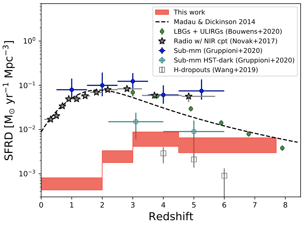
Figure 1: The star formation rate density diagram, including many literature measurements focusing on the early universe (z > 3). The results from this paper indicate that a missing population of galaxies might account for a large portion of the SFRD at z > 4. [Talia et al. 2021]
Observing star formation rates during the first 2 billion years of the universe (z > 3) is incredibly difficult. Not only were the first galaxies intrinsically smaller and fainter than galaxies we see today, but starting at z ~ 6, the universe is pervaded by a dense fog of neutral hydrogen (from which galaxies formed!) that obscures their light. Given these difficulties, these incredibly early galaxies are only now being observed in large numbers.
The authors of today’s paper point out that the existing samples of z > 3 galaxies are not at all representative. For the most part, and almost exclusively at z > 6, these galaxies are discovered via their bright ultraviolet (UV) emission, which has been redshifted so that it is observed in the optical and infrared. Not only must these galaxies be incredibly bright to be found at such large distances, but their intensive UV emission translates directly to an enormous star formation rate. That is, the feature that makes them easy to find also makes their star formation rates high. This is a huge bias in our samples! To overcome this bias, the authors turn to radio wavelengths. They used a large radio survey VLA-COSMOS to find 197 radio sources that have no counterpart in near-infrared wavelengths. These, they argue, are heavily dust-obscured galaxies without any UV emission — the missing link.

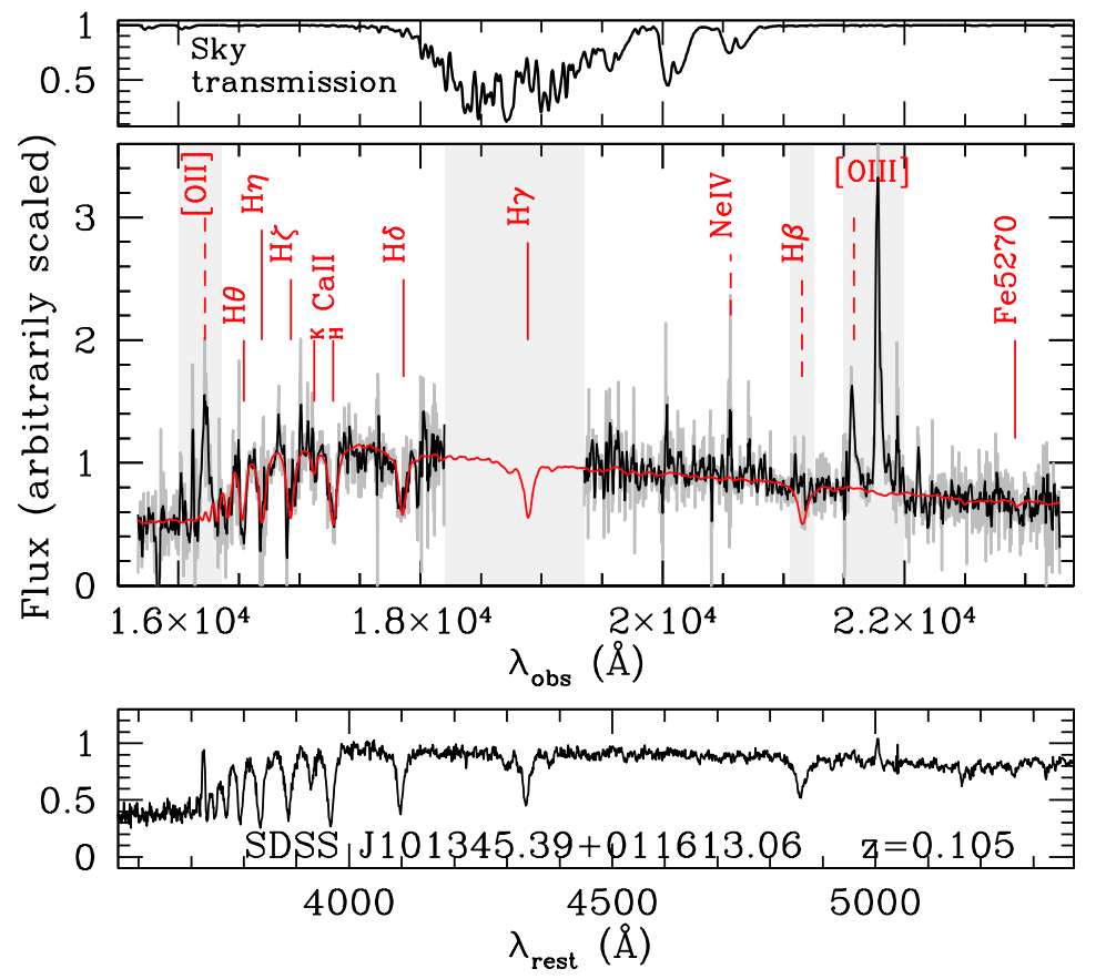
Figure 2: Median galaxy template (top) fitted to stacked observations in many broadband filters (bottom). The derived average physical parameters, as well as the redshift distribution, are also shown. [Talia et al. 2021]
The authors’ first test was to stack the broadband brightness measurements of each galaxy together so that they can predict what the average total spectrum would look like for these galaxies, and hence their average properties. The lack of blue light on the left-hand side of the spectrum indicates that there is no luminous UV component as seen in the UV-bright galaxies of previous samples. Moreso, the authors estimate an incredibly high dust extinction of a whopping 4.2 magnitudes (nearly a factor of 50)! These galaxies are super dusty indeed.
Using a similar approach to the stacked analysis, the authors then estimate the redshift and star formation rate for each of the 98 galaxies for which they could reliably measure an infrared brightness. Due to their unique radio selection approach, the authors are able to compile a large sample of very high redshift galaxies at z > 4.5. They estimate the redshifts and star formation rates for the remaining 99 sources as well, but with much greater uncertainty.
Lastly, the authors compute the SFRD using their sample, taking care to correct for any dusty galaxies they may have missed. This is a challenging correction to make, so the authors do so by adopting an agnostic approach, seeing how their SFRD looks depending on how complete their sample might be.
As shown by the red bars in Figure 1, it is precisely this population of highly dust-obscured galaxies at z > 3, invisible to optical and infrared surveys, that may indeed constitute a significant portion of the star formation rate density in the early universe compared to other less-dusty samples!
These findings highlight the surprising extent of our missing knowledge of the first galaxies, and they encourage investment in future radio surveys with ALMA and follow-up with JWST.
Original astrobite edited by William Saunders with Lukas Zalesky.
About the author, John Weaver:
I am a second year PhD student at the Cosmic Dawn Center at the University of Copenhagen, where I study the formation and evolution of galaxies across cosmic time with incredibly deep observations in the optical and infrared. I got my start at a little planetarium, and I’ve been doing lots of public outreach and citizen science ever since.