
Polarime-trying to Map Magnetic Fields in the Orion Nebula
Editor’s note: Astrobites is a graduate-student-run organization that digests astrophysical literature for undergraduate students. As part of the partnership between the AAS and astrobites, we occasionally repost astrobites content here at AAS Nova. We hope you enjoy this post from astrobites; the original can be viewed at astrobites.org.
Title: HAWC+/SOFIA Multiwavelength Polarimetric Observations of OMC-1
Authors: David T. Chuss et al.
First Author’s Institution: Villanova University
Status: Published in ApJ
OMC-What?
The Orion Molecular Cloud 1 (OMC-1) is part of the Orion Nebula, and one of the most massive star-forming regions in the solar neighborhood. The gas and dust within OMC-1 act as a nursery for young stars, providing them with the necessary materials to develop. As such a close and large stellar nursery, OMC-1 is an easily accessible and important laboratory for studying the still-mysterious conditions that surround and encourage star formation. Today’s paper contributes to our understanding of star formation by determining OMC-1’s magnetic field and dust properties using polarimetry (more on this technique later!).
OMC-1 is a particularly interesting target for magnetic field and dust measurements because of the variation in structure across the cloud, which is shown in Figure 1. In front of OMC-1, there is an HII region ionized by a relatively young group of stars, the Trapezium cluster. The west side of OMC-1 hosts the Kleinman-Low (KL) Nebula and the Becklin-Neugebauer (BN) object. The KL Nebula is a clump of molecular gas and dust with a bunch of massive stars inside, of which the BN object is the brightest. In the infrared, the KL Nebula appears to be exploding because stellar winds from the massive stars heat up the surrounding gas. The southeast region of OMC-1 contains the Orion Bar, a photodissociation region that is cold, neutral, and creates the divide between HII and molecular gas. These features contribute to a complex magnetic field structure within OMC-1 that today’s authors map with polarimetry measurements.
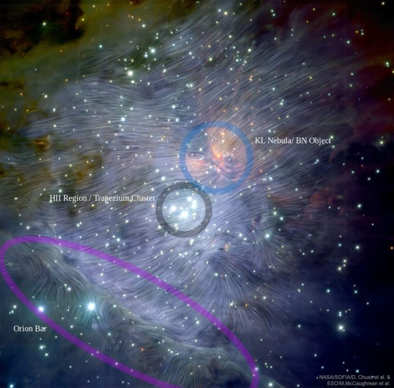
Figure 1: The OMC-1 region, with overlaid magnetic field lines. Blue shows the KL Nebula and BN object, gray shows the HII region ionized by the Trapezium cluster, and purple shows the Orion bar. [NASA/SOFIA/D. Chuss et al. & ESO/M. McCaughrean et al.]
So What Is This Polarimetry I Speak Of?
We’ve all heard of polarized sunglasses, which block sunlight and reduce glare. Thinking of light as a wave, it travels in one direction and oscillates in the two planes perpendicular to that direction of travel. Polarized sunglasses block out one of these planes of vibration, and allow only half of the light to travel through the lenses.
Polarization measurements in astronomy work much the same way. For today’s paper, we are looking at the infrared light that is emitted from dust, but stars and other sources can emit polarized light too. For dust, the primary concepts of polarization remain the same as the case of blocking light with sunglasses. However, instead of blocking the light, dust actually emits light that has one plane of vibration brighter than the other from the start. To understand the reason behind this, assume that the dust has an egg shape. Because there is more surface area along the long axis of the egg than the short axis, we get more emission traveling in the direction of the long axis. This creates a net polarization of the signal: we get more infrared light in the direction that is parallel to the long axis of the dust. Lots of theories suggest that dust aligns its long axis perpendicular to the magnetic field, so by measuring the direction of the polarization, we can infer the direction of the magnetic field!
Flying High
Today’s authors used the HAWC+ instrument onboard NASA’s airborne observatory (the Stratospheric Observatory for Infrared Astronomy, or SOFIA) to look at the infrared emission of the dust in OMC-1. They measured the total flux and polarization at four different wavelengths, and the results of their measurements can be seen in Figure 2. Interestingly, they found that at the smaller wavelengths (upper two panels), the magnetic field direction near the BN/KL objects, represented by the white star, is radically different than the surrounding region. The authors also discovered that the magnetic field direction in the Orion Bar differs significantly from elsewhere in OMC-1, and the magnetic field strength and dust temperature are highest near the BN/KL explosion location.
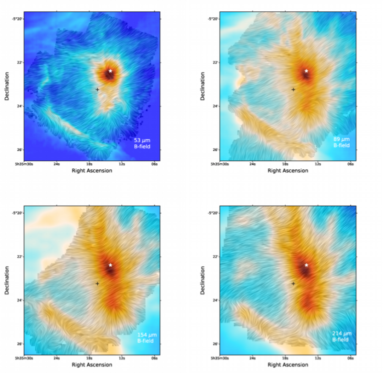
Figure 2: Polarimetry measurements at 53, 89, 154, and 214 microns. The star symbol represents the location of the BN object, while the Orion Bar can be seen at the lower left. Colors represent total intensity, with red the highest and blue the lowest. Lines represent magnetic field direction. Click and zoom in to notice the change in the magnetic field with wavelength near the BN object! [Chuss et al. 2019]
Sweeping (Up the Dust) Conclusions
So why the change in magnetic field direction and strength across the OMC-1 region? The authors propose some interesting explanations. Remember how the KL nebula appears to be exploding from stellar winds? Well, it’s possible that this explosion has compressed the magnetic field opposite the material that it spits out, creating the distinctly different direction of the magnetic field that we see at shorter wavelengths. And the reason we don’t see the same compression at longer wavelengths? Longer wavelengths are emitted by the colder dust (Wein’s Law) that is likely to be outside of the explosion range! The authors also provide an explanation for the change in magnetic field direction that is present in the Orion Bar: the magnetic field of the bar may run parallel to its long side. When the vector of the magnetic field along the bar is added to the vector of the magnetic field in the surrounding region, it is likely to cancel itself out.
These insights on the magnetic field structure of OMC-1 demonstrate the power of polarimetry in astronomy, and the HAWC+ instrument on SOFIA will continue to make similar measurements more prevalent for molecular clouds. Because molecular clouds act as stellar nurseries, learning about their properties (like the direction and strength of their magnetic field) provides us with a better understanding of star formation processes.
About the author, Ashley Piccone:
I am a second year PhD student at the University of Wyoming, where I use polarimetry and spectroscopy to study the magnetic field and dust around bowshock nebulae. I love science communication and finding new ways to introduce people to astronomy and physics. In addition to stargazing at the clear Wyoming skies, I also enjoy backpacking, hiking, running and skiing.

![AGN luminosity vs [OIII]](https://aasnova.org/wp-content/uploads/2020/05/HIPS-Fig-2.png)


 Ships")

