Editor’s Note: Astrobites is a graduate-student-run organization that digests astrophysical literature for undergraduate students. As part of the partnership between the AAS and astrobites, we occasionally repost astrobites content here at AAS Nova. We hope you enjoy this post from astrobites; the original can be viewed at astrobites.org.
Title: Tilted Circumbinary Planetary Systems as Efficient Progenitors of Free-Floating Planets
Authors: Cheng Chen et al.
First Author’s Institution: University of Leeds
Status: Published in ApJL
All planets orbit stars.
Okay, that was a lie. But a hundred years ago, it seemed super true — we only knew of the planets around our own Sun.
Then, later, it still seemed decently true. Astronomers started finding planets around other stars in the 1990s (which the opening statement supported!). At this point, though, the field had at least begun to consider that there could be a population of “free-floating planets”: planet-sized bodies wandering through space, unaffiliated with any particular star.
Because our methods of finding planets, at that point, relied on the dimming or shifting of a host star’s light, these rogues seemed unknowable (if they existed at all). So perhaps the statement could be modified to read “all planets that we can detect orbit stars,” which would still maybe hold a little truth.
As our telescopes (and our techniques) have improved, though, it has become very clear that the statement is… irredeemably untrue. Since the turn of the century, largely through a more direct observational technique called microlensing, we’ve gradually uncovered a rich population of free-floating planets dancing in the vast cosmic dark. (Just in the past few months, JWST revolutionized yet another sub-field with its discovery of free-floating pairs of planets, but that’s a topic for another ’bite.)
Young, Wild, and Free: The Instability of Newborn Planetary Systems
But where do these unbound beauts come from? There are a few proposed mechanisms, but one of the most likely methods involves planets forming around stars (like normal!) but subsequently being violently ejected from their bound orbits.
The period immediately following the formation of the planets is often suspected to be pretty messy. In the solar system, we think there was a major instability right after planets formed, in which our eight major planets interacted strongly with each other before settling into roughly the orbits they have today.
In fact, simulations of such an instability suggest that there could have originally been a fifth giant planet in the outer solar system, formed alongside Jupiter, Saturn, Uranus, and Neptune. During the period of unrest (often called a “late instability” due to its occurrence after planet formation was complete), this planet would have been “kicked” off of its original orbit — and ejected from the solar system altogether — through interactions with the other giants. Any such planet would, at this point, be a free-floater.
Today’s article talks about these sorts of “planet–planet scattering” ejections, but it doesn’t talk about the solar system (nor any particular observed planetary system). Instead, in a common theorist tactic, the authors consider a whole class of planetary systems: those existing around two stars rather than one.
Two Stars Are Better than One (for Planetary Ejections)
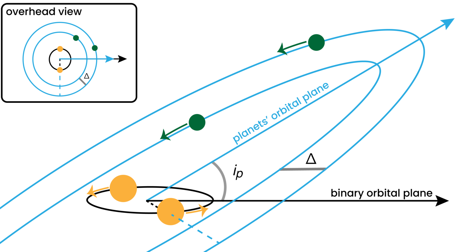
Just as planets can orbit stars, stars can orbit each other. And if their orbit is small enough, protoplanetary disks — and, thereafter, planets — can form around the pair of them. One of the most famous (fictional) examples of such a system is Star Wars’ Tatooine, which enjoys an iconic double sunset courtesy of the binary stars around which it orbits. A diagram of planets orbiting a pair of stars is shown in Figure 1.

Figure 1: In the setup described in this work, two planets (green) orbit around a binary pair of stars (yellow). The planets’ orbits are separated by a dimensionless distance parameter Δ — the distance between the orbits in terms of their mutual sphere of influence. The orbits start off aligned with each other (though this can change over the course of a simulation!), but they aren’t necessarily aligned with the orbit of the stellar binary. The authors test the stability of systems spanning a range of different inclinations (ip) and separations (Δ). [Mark Dodici]
Ejections in planetary systems around
single stars, though possible, probably don’t happen often enough to explain how common free-floating planets are. In dynamics, things can get a lot more complicated when you add just one extra body (see, e.g.,
the n-body problem!), so the authors of today’s article wonder if adding another star will provide enough complication to eject more planets.
(This isn’t an unreasonable addition; binary pairs — and even binaries close enough to allow for planet formation — make up a significant fraction of all stars, so they’re definitely worth modeling.)
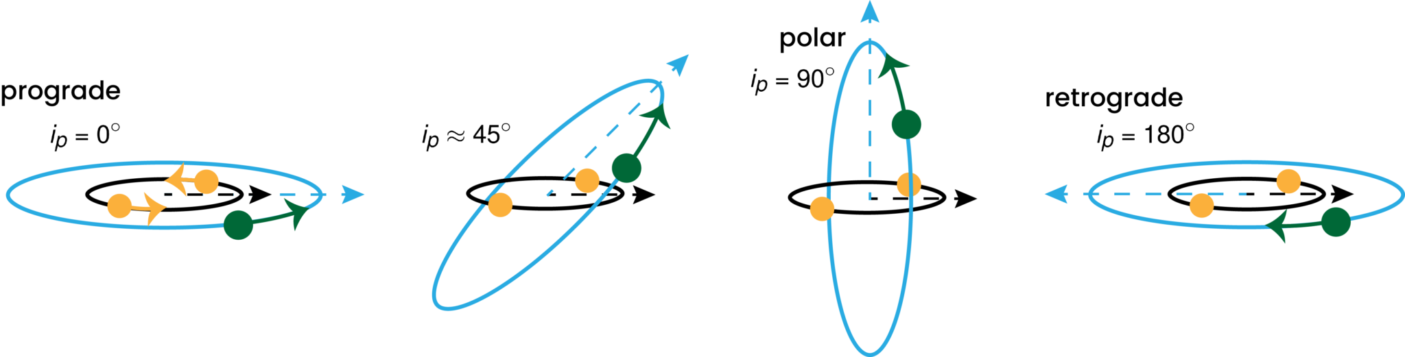
Specifically, the authors simulate planetary systems where two planets, separated by some distance, trace out orbits that are inclined relative to the orbit of the central binary stars. (See Figure 2 for examples of different orbital inclinations.) They test systems with a range of initial inclinations, for a range of planet separations, for a select few choices of unequal planet masses. Through these simulations, they cover a broader range of parameter space — i.e., the ranges of values that a real-life system could have for its properties — than previous work.
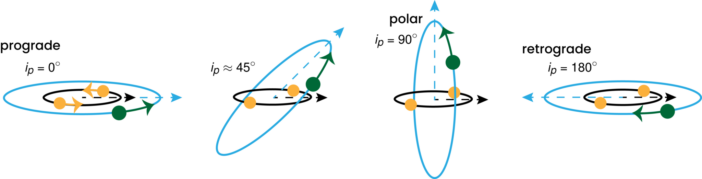
Figure 2: Examples of planetary systems with a few different inclinations, from prograde to retrograde. From this work, the orbits that most commonly lead to ejections are neither prograde, nor polar, nor retrograde — that is, systems with ip ≈ 45° see ejections most often. [Mark Dodici]
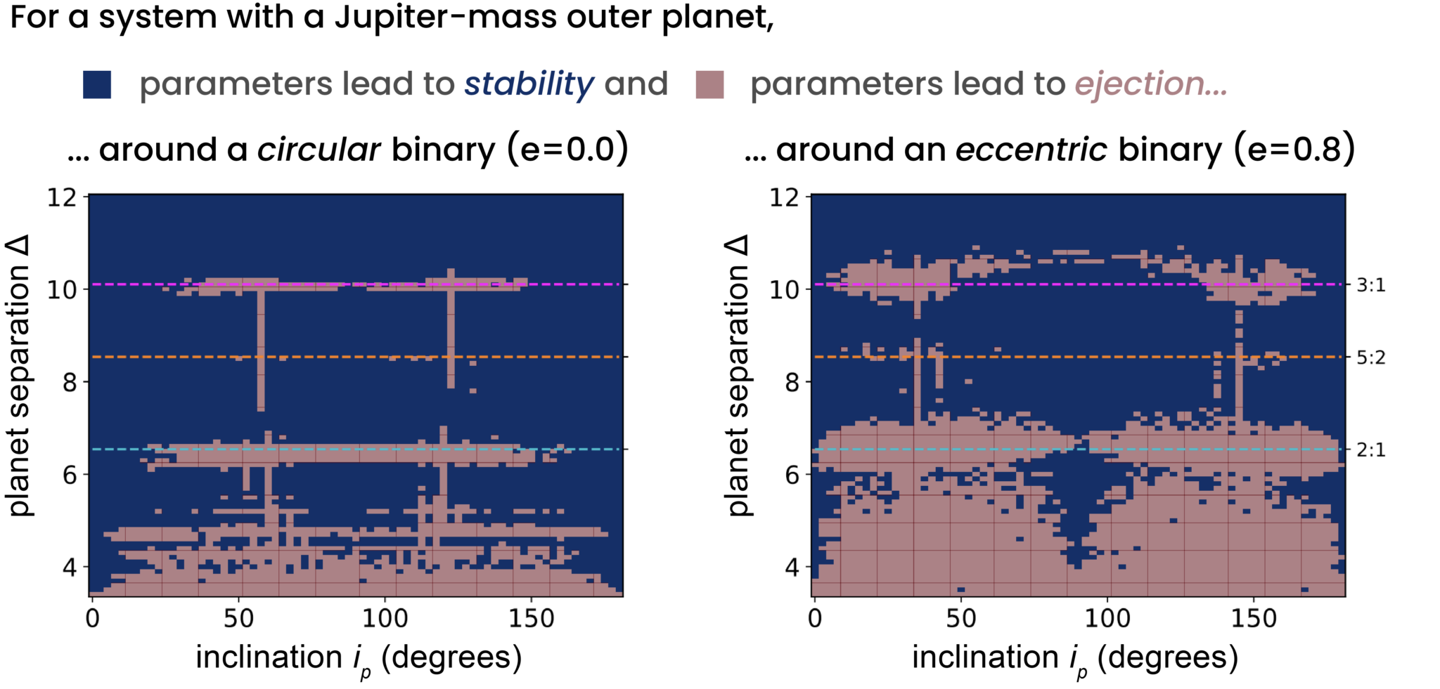
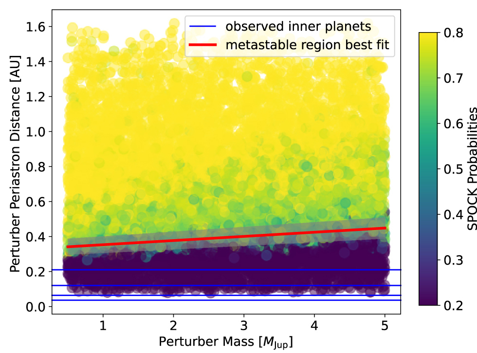
For all planet masses, the systems most likely to yield ejections involve close-together planets with orbits that are neither well-aligned (“prograde” or “retrograde”) nor perpendicular to the binary (“polar”). (Results are presented in Figure 3.) Systems are much more likely to yield ejections when they have at least one planet more massive than Neptune, though the less-massive planet, if there is one, is always the one ejected.
Eccentric binary stars — those orbiting each other on oblong, elliptical paths rather than perfect circles — also boost the ejection rate of the planets around them.
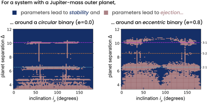
Figure 3: For a given system, the authors reported whether each set of parameters was stable (blue) or resulted in an ejection (light red). On the left, we see a range of systems with different inclinations and planet separations around circular binaries. On the right, we see the same range of inclinations and separations around eccentric binaries, with e = 0.8. All systems in these plots have a Jupiter-mass outer planet with an Earth-mass planet orbiting interior to it. Dashed, colorful lines on these plots point out a few mean motion resonances (see text), which are known to be unstable in tilted planetary systems. In the article, the authors show similar plots for different combinations of planet masses; these generally show similar trends in ejection vs. stability for various inclinations and separations. [Adapted from Chen et al. 2024]
There are some fun planetary dynamics underlying these results! From the basic law of gravity, we know that more-massive, closer planets have more of an impact on others in their own system; it makes sense, then, that more-massive, closer planets cause more ejections. Oddly inclined orbits (i.e., not prograde, polar, or retrograde) often lead to long-term oscillations in inclination; if the two planets take on
different inclinations over the course of their lifetime,
von Zeipel-Kozai-Lidov cycles can sometimes increase their eccentricity until one of them becomes unbound. And although ejections were most common among close-together planet pairs, they aren’t impossible with a bigger gap; instability can occur near
mean motion resonances, where the periods of the two planets are integer multiples of each other (e.g., at the 2:1 resonance, the inner planet orbits twice as quickly as the outer).
A Few More Free-Floaters
That all said, this isn’t an article about planetary dynamics — it’s about free-floating planets. These results show that a decent variety of planets can be ejected from planetary systems around binary stars, yielding a decent total occurrence rate for free-floaters from this mechanism. This is a decent win for planet–planet scattering as a potential source of unbound planets!
As in any theory article, there’s work to be done to constrain exactly how often we expect these Tatooine-like systems to eject planets, as well as the range of masses we would expect these ejected planets to have. And in reality, the total population of free-floating planets almost certainly comes from some combination of several effects, each contributing their own subpopulations. But with recent and upcoming observations from Subaru Hyper Suprime-Cam, TESS, Roman, and JWST, there will certainly be no lack of data to which models like these can be compared.
Original astrobite edited by Sahil Hedge.
About the author, Mark Dodici:
Mark is a PhD student in astronomy and astrophysics at the University of Toronto. His space-based interests include planetary systems, from their births to their varied deaths, as well as the dynamics of just about anything else. His Earth-based interests include coffee, photography, and a little bit of singing now and again. You can follow him on X (@MarkDodici) or on BlueSky (@dodici.bsky.social).


