
Does Active Galactic Nucleus Feedback Cause Our Universe to Take a Cosmic Afternoon Nap?
Editor’s Note: Astrobites is a graduate-student-run organization that digests astrophysical literature for undergraduate students. As part of the partnership between the AAS and astrobites, we occasionally repost astrobites content here at AAS Nova. We hope you enjoy this post from astrobites; the original can be viewed at astrobites.org.
Title: Distinguishing Active Galactic Nuclei Feedback Models with the Thermal Sunyaev–Zel’dovich Effect
Authors: Skylar Grayson et al.
First Author’s Institution: Arizona State University
Status: Published in ApJ
Let’s imagine the evolution of the universe as a regular day on Earth. If the Big Bang was when the clock struck midnight, then the cosmic “dawn” is when the first stars and galaxies started to light up our universe. After the cosmic dawn ended, galaxies continued to form stars and grew rapidly throughout the morning. Around cosmic “noon,” most galaxies in our universe were huge and even hosted massive black holes at their centers. However, as the afternoon rolled by, the universe seems to have gotten pretty lethargic in forming stars and expanding galaxies. Looks like the universe is fond of taking an afternoon siesta!
What caused the rapidly forming galaxies in the universe to suddenly slow down and stop star formation? Why didn’t they continue growing to bigger and bigger sizes? Some astronomers believe this cosmic downsizing is due to feedback from active black holes (also known as active galactic nuclei). This feedback typically occurs when the black hole spews out fast winds called outflows that contain gas and dust and expel it to large distances, sometimes far beyond the galaxy itself. Such outflows can clear the galaxy of any star-forming gas and effectively shut down star formation.
There is still much mystery around exactly how the active galactic nucleus feedback affects star formation in the galaxy. Nevertheless, various feedback models are often incorporated into simulations of galaxy formation to understand how the universe evolved. This leads to contrasting theories of galaxy evolution, so comparing the simulation feedback models to actual observations of feedback effects is essential to improve our understanding of active galactic nucleus feedback.
It is hard to directly observe an active galactic nucleus outflow, as they can be as fast as thousands of kilometers per second and cannot be captured instantaneously. Instead, we can look for indirect evidence. Our universe is filled with a microwave background believed to be a remnant of the primordial universe. If we have some high-energy electrons from gas heated by a powerful activity, such as a black hole ejecting material, they would possibly interact with the low-energy photons from the cosmic microwave background and give the low-energy photons a slight boost. This effect, known as the thermal Sunyaev–Zeldovich effect, is a good clue of a possible active galactic nucleus feedback episode.
The authors of today’s research article set out to do look for this indirect evidence of active galactic nucleus feedback. They compare observations of galaxies with signals from the thermal Sunyaev–Zeldovich effect and signals produced by galaxy simulations with and without active galactic nucleus feedback. This can help them determine if the simulations correctly model feedback and if this feedback accurately explains the observed cosmic downsizing.
Comparing Simulations vs. Observations
The authors generate maps of the thermal Sunyaev–Zeldovich effect signal from SIMBA, which is a simulation that explores the co-evolution of galaxies and black holes. They generate one set of maps with galaxies that have active galactic nucleus feedback and another set with no feedback. They highlight a sub-sample of galaxies from the former as quiescent or galaxies that have shut down and have no ongoing star formation. There are plenty of such galaxies in the universe, and they are likely there because active galactic nucleus feedback completely removed all the gas in the galaxy and thus permanently halted star formation.
The thermal Sunyaev–Zeldovich effect can be detected in observations by looking for distortions in the cosmic microwave background from data collected by radio telescopes. (The photons of the cosmic microwave background have low energies and thus need telescopes sensitive to long wavelengths of light to study them.) The authors take radio data of a similar sample of galaxies with active galactic nuclei (including quiescent galaxies) and without. They do this at two different redshifts, z = 1 and z = 0.5. The authors matched the simulated data with suitable observational effects so they could be compared realistically.
The Compton y-parameter is then used to compare the observed signal to the simulated signal. The Compton y-parameter is defined as the number of scatterings multiplied by the energy gained per scatter instance and is a commonly used term to characterize scattering in a system. As seen in Figure 1, at z = 1, the observed data match well with the quiescent active galactic nucleus model and the active galactic nucleus model in general. The data do not line up well with the no active galactic nucleus (i.e., no feedback) model, indicating that the feedback incorporated by the simulation is successful at replicating observed properties at these redshifts.
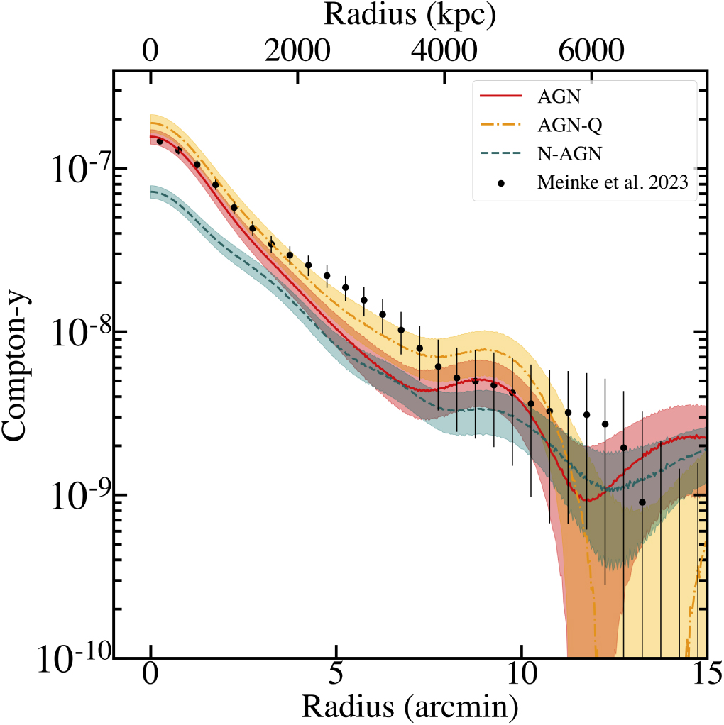
Figure 1: A comparison of observed and simulated thermal Sunyaev–Zeldovich signals at a redshift of z = 1. The observed data (black points) agree with the active galactic nucleus feedback model. [Grayson et al. 2023]
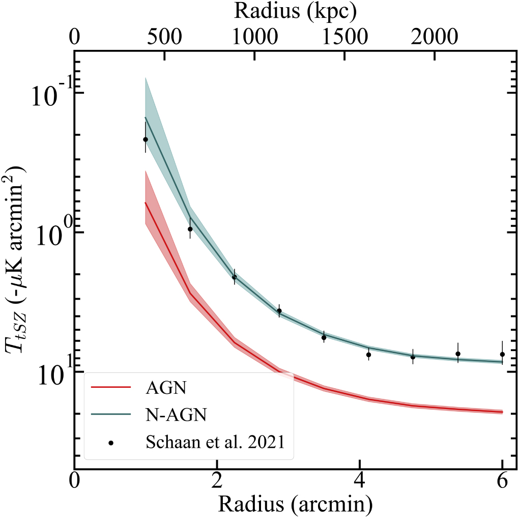
Figure 2: A comparison of observed and simulated thermal Sunyaev–Zeldovich signals at a redshift of z = 0.5. The observed data (black points) do not agree with the active galactic nucleus feedback model, but this is likely because the feedback is modeled incorrectly in the simulations. [Grayson et al. 2023]
Original astrobite edited by Jack Lubin.
About the author, Archana Aravindan:
I am a PhD candidate at the University of California, Riverside, where I study black hole activity in small galaxies. When I am not looking through some incredible telescopes, you can usually find me reading, thinking about policy, or learning a cool language!


