Features RSS

planet orbiting K dwarf

Signs of life in planetary atmospheres are hard to spot! A new study suggests that the best strategy for discovering them may be to look at planets orbiting K-dwarf stars.

The Hunt for Fingerprints

Is there life beyond Earth? This remains one of the most profound scientific questions astronomers are currently poised to address, and development of ever more powerful telescopes continues to bring us closer to an answer.

One way we can hope to use these telescopes to identify the presence of life on distant exoplanets is by detecting atmospheric biosignatures. Left alone, a planet’s atmosphere ought to be in chemical equilibrium. But when life is present, the atmosphere accumulates excess gases produced by the life — telltale fingerprints that we can hope to spot.

Signatures in Methane

stellar spectra

The spectra of various types of stars used by the author in models, including the Sun (a G2V dwarf) and three types of K dwarfs. K dwarfs produce less radiation in the 200–350 nm range. [Adapted from Arney 2019]

A good example of these fingerprints is the simultaneous presence of oxygen and methane in a planet’s atmosphere — something that shouldn’t occur if life isn’t there. The hunt for this biosignature is complicated by the fact that methane in the presence of oxygen is destroyed via chemical reactions driven by stellar light; if too much of the methane is removed by these photochemical reactions, we won’t be able to detect it.

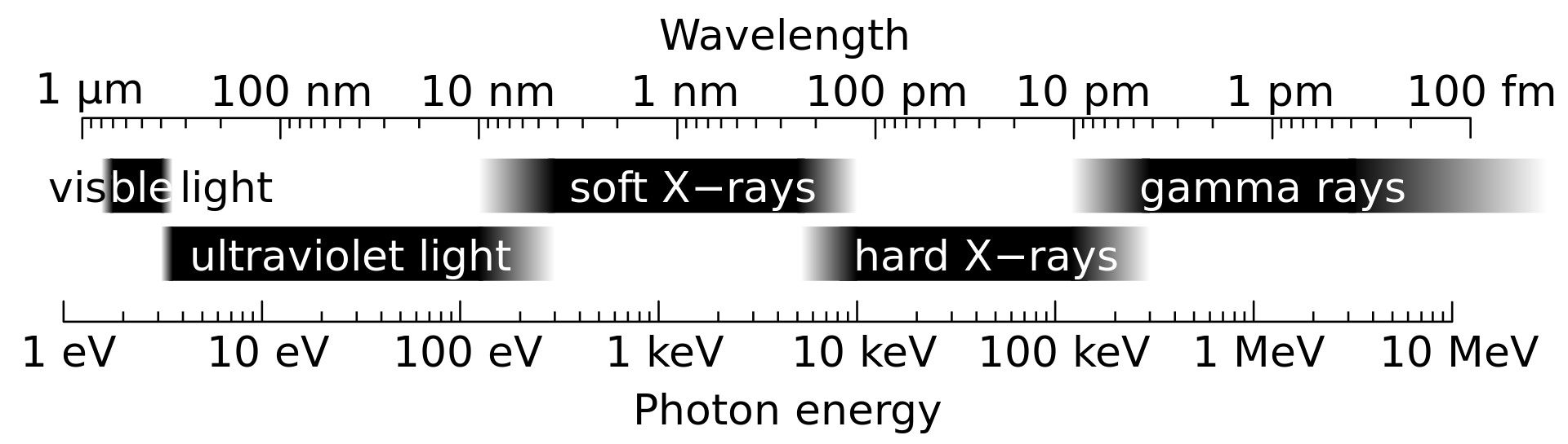
There’s hope, though: some planets may be more likely to maintain life-produced methane in their atmospheres than others. Stellar light in the 200–350 nm range triggers this reaction — so the less light a planet’s host star produces in this range, the longer methane can survive in the planet’s atmosphere. This means that the type of host star matters: G dwarfs like the Sun will destroy the methane in their planets’ atmospheres faster than smaller and cooler M dwarfs.

Model planet spectra

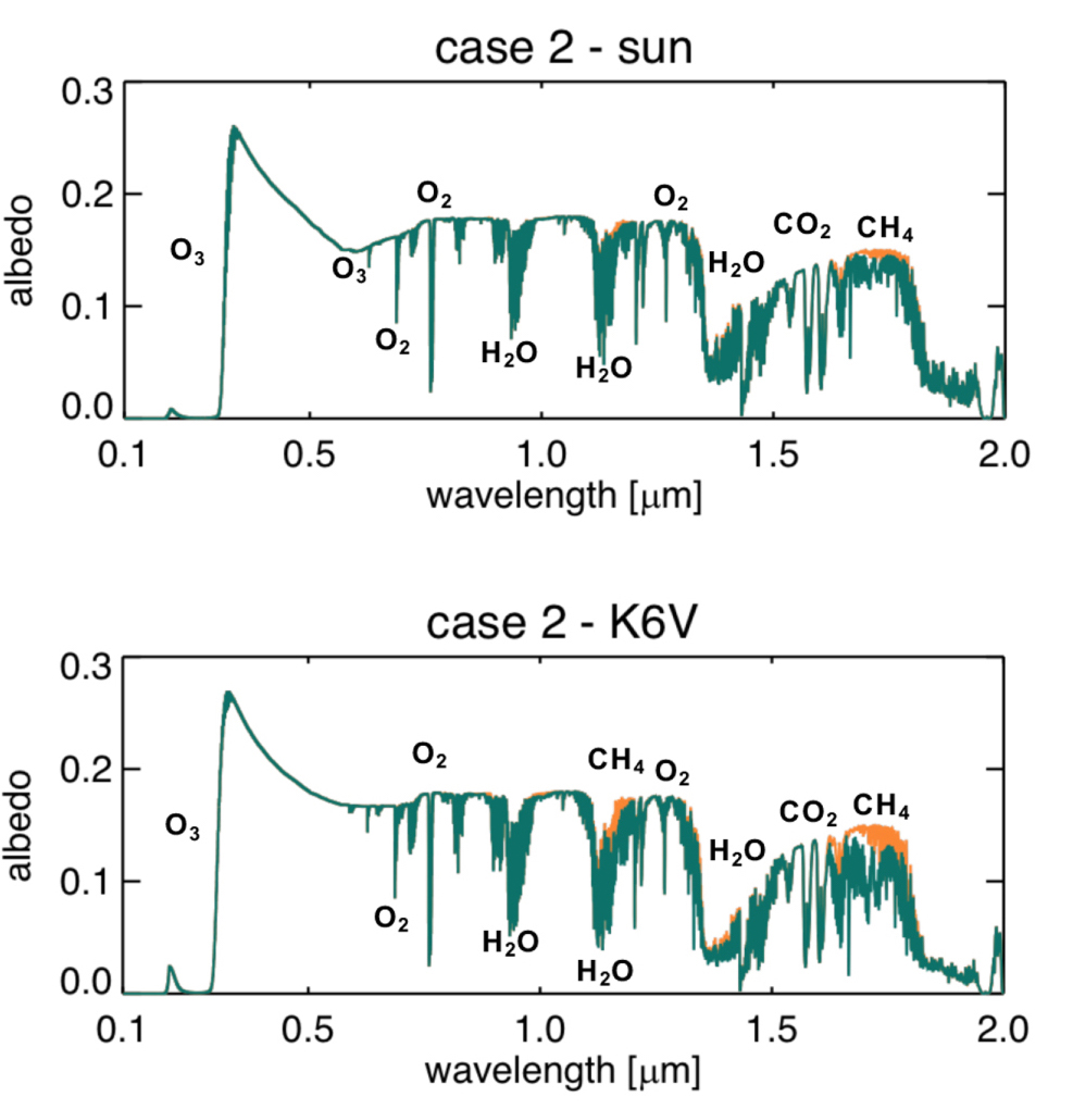
Spectra from two of the author’s modeled quasi-modern planets: one around the Sun, and one around a K6V star. Orange lines show the spectra with methane removed, making the methane absorption features easier to see. The absorption features are much more evident in the planet around the K dwarf. [Adapted from Arney 2019]

Unfortunately, M dwarfs have other complications hindering the potential for life — including high levels of stellar activity that drive atmospheric loss from their planets. For this reason, scientist Giada Arney (NASA Goddard SFC and NASA NExSS Virtual Planetary Laboratory) has explored the advantages of a different type of star: K dwarfs.

The K-Dwarf Advantage

K dwarfs fall between G and M dwarfs in size and temperature, and they are more abundant than G dwarfs. Dimmer than G dwarfs, K dwarfs provide better planet-to-star contrast ratios that make it easier to observe potential habitable worlds. And they are are less active than M dwarfs, providing a more hospitable environment for their planets.

In addition to these benefits, K dwarfs also produce less radiation in the 200–350 nm range than G dwarfs do. By using a one-dimensional photochemical climate model to simulate a variety of planetary atmospheres, Arney demonstrates that a planet orbiting a K6V star can support roughly an order of magnitude more methane in the presence of oxygen relative to an equivalent planet around a G2V dwarf like the Sun.

starshade

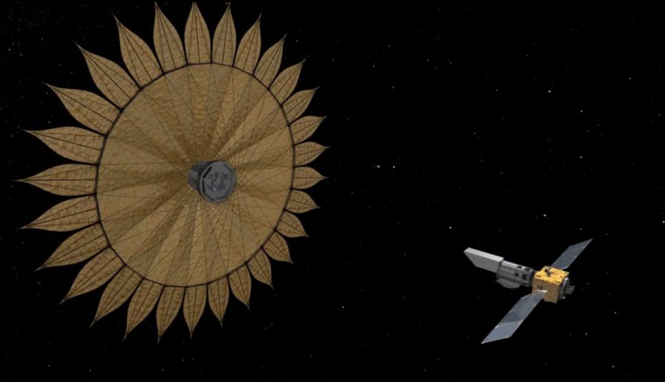
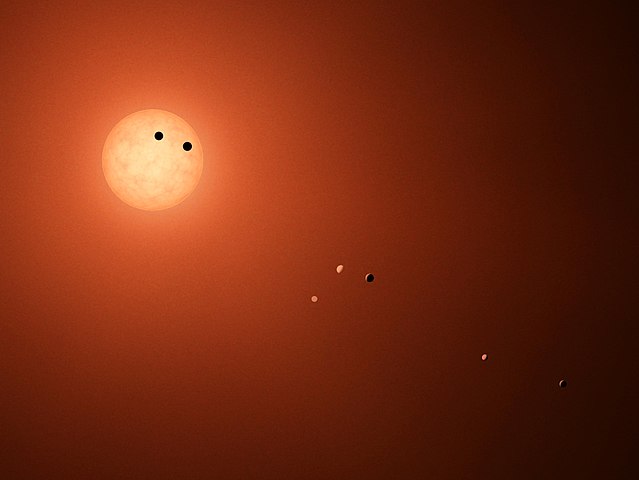
Artist’s impression for one possible configuration of the proposed HabEx mission, in which a starshade could be used to help better image distant exoplanets. [NASA/JPL/Caltech]

But is this enough to produce signatures we can soon detect? Arney uses synthesized spectra to show that, with the technologies proposed for potential future missions like LUVOIR or HabEx, we have a decent chance of spotting the simultaneous methane and oxygen signatures in planets orbiting nearby mid-late K-dwarf stars. Thus the “K-dwarf advantage” gives us a great list of promising targets for the next major space missions!

Citation

“The K Dwarf Advantage for Biosignatures on Directly Imaged Exoplanets,” Giada N. Arney 2019 ApJL 873 L7. doi:10.3847/2041-8213/ab0651

Centaurus A

What’s going on in our high-energy sky? Powerful phenomena abound in our universe, and they can produce photons with tremendous energies. A new study explores a high-energy mystery from one of these sources: active galactic nuclei, or AGN.

gamma-ray spectrum

Gamma rays span a broad range of energies in the most energetic part of the electromagnetic spectrum. Very high-energy gamma rays initially emitted from AGN have energies above 100 GeV, but these are reprocessed by interactions with background photons to energies of 1–100 GeV. [Ulflund]

Where Are the Gamma Rays?

Active galactic nuclei — the accreting supermassive black holes lurking at the centers of some galaxies — dot our universal landscape, spewing out very high-energy gamma-ray photons within jets moving at nearly the speed of light. These energetic photons speed across the sky — but they don’t travel unencumbered.

Theory predicts that this energetic emission should be effectively reprocessed as it slams into the cosmic microwave background, generating a compact sheath of gamma-ray emission in the 1–100 GeV range, beamed forward in the direction of the jets emitted from each AGN. But there’s a problem: we don’t see this expected flux.

AGN sources

Galactic coordinates of the sources used to generate the authors’ stacked analysis. Two types of AGN-containing galaxies are included: FR I and FR II galaxies. [Broderick et al. 2019]

One possible explanation for the missing light is that these traveling photons could be deflected from their path by a strong, large-scale magnetic field threading through intergalactic space. This would convert the compact, forward-beamed sheath into a more diffuse, harder-to-spot gamma-ray halo around each AGN. In a new study, a team of scientists led by Avery Broderick (University of Waterloo and the Perimeter Institute for Theoretical Physics, Canada) has gone on the hunt for these missing gamma-ray halos.

Stacks of Galaxies

Though the proposed gamma-ray halos may be too faint to spot individually, Broderick and collaborators suggest that by stacking a bunch of gamma-ray observations of off-axis AGN on top of one another, we should easily be able to detect their combined halo — if it exists.

radio jet alignment

The process of aligning the jets in two different radio images: an FR I galaxy (top) and an FR II galaxy (bottom). [Broderick et al. 2019]

To do this, the AGN must first be oriented in the same direction. Broderick and collaborators use radio observations of AGN jets pointed off our line of sight to identify each jet’s orientation. They determine the transformations needed to align each of the radio jets, and then apply this transformation to corresponding Fermi-telescope gamma-ray observations of the active galaxies. The result is a sample of nearly 9,000 gamma-ray observations of AGN, all oriented in the same direction.

Broderick and collaborators then stack these observations and compare their results to a model of what we would expect to see if an intergalactic magnetic field were deflecting the gamma-ray photons, generating a faint halo around the AGN.

Still No Halos

gamma-ray halos

Top: the authors’ stacked gamma-ray observations for FR I (left) and FR II (right) galaxies. Bottom: the expected signals if gamma-ray halos were present. The observations clearly rule out the presence of faint halos. [Broderick et al. 2019]

Intriguingly, the authors find no hint of a combined gamma-ray halo. Their non-detection places strict limits on the strength of the intergalactic magnetic field allowed in this picture, and it rules out magnetic fields as an explanation for why we don’t see the gamma rays we expect from AGN.

What does this mean? Broderick and collaborators argue that this requires us to consider brand new physics in high-energy processes. There must be some unexpected mechanism that prevents the creation of the expected gamma-ray halos, either because the highest-energy emission is suppressed in gamma-ray bright AGN, or because some process affects this emission before it can lead to the generation of halos. The mystery deepens!

Citation

“Missing Gamma-Ray Halos and the Need for New Physics in the Gamma-Ray Sky,” Avery E. Broderick et al 2018 ApJ 868 87. doi:10.3847/1538-4357/aae5f2

Galactic center in infrared

How does a supermassive black hole affect its stellar neighbors? One way to explore this question is by searching for old, giant stars in the extreme environs of the galactic center.

Crowded Quarters

Galactic center in visible light

Dark dust lanes block the visible light from the galactic center, hiding the dense star cluster located there. [Dave Young]

The supermassive black hole at the center of our galaxy likely plays a huge role in the evolution and dynamics of stars in its neighborhood, as well as in how they are spatially distributed.

Theory predicts that old, giant stars near the galactic center should be arrayed in a “cusp”-like distribution, with the number of stars per square arcsecond increasing sharply toward the central black hole. Faint red giants seem to follow the expected distribution, but brighter red giants — which can be probed closer to the center of the galaxy — do not. Instead, these stars appear to follow a “core”-like distribution, with fewer stars than expected within the central arcsecond of the galaxy.

Many theories have been proposed to explain the apparent lack of bright red giants near the galactic center, from stellar collisions to tidal disruption by the supermassive black hole. While these factors may play a role, it’s also possible that observational challenges have prevented astronomers from fully cataloging the stellar population at the galactic center.

Habibi et al. 2019 Fig. 2

Giant stars from this study (black stars) on an H-R diagram with the theoretical isochrones used to determine the stellar ages. [Habibi et al. 2019]

Tracking Down Missing Stars

Observing stars so close to the galactic center is tricky — it’s crowded there, and starlight is highly extincted by dust clouds in the galactic plane at many wavelengths. In order to probe the stellar population near the galactic center, a team led by Maryam Habibi (Max Planck Institute for Extraterrestrial Physics, Germany) analyzed more than a decade’s worth of near-infrared stellar spectra from the SINFONI spectrograph on ESO’s Very Large Telescope.

The spectra used in this study were collected with the help of adaptive optics, in which the telescope’s mirror is deformed slightly to correct for the effects of turbulence in Earth’s atmosphere in close to real time — critical for observations of individual stars in a field as crowded as the galactic center!

By co-adding multiple epochs of spectra to tease out faint spectral features, the authors derived the effective temperature, spectral type, age, mass, and radius for each target star. Their deeper spectra allowed them to identify old giants that had previously been misclassified as younger stars, bringing the number of known giants to 21.

Habibi et al. 2019 Fig. 4

Observed stellar density profiles from this and other studies of the galactic center. Previously, the observed distribution was consistent with a core-like profile (blue dashed line). The inclusion of the newly identified giants shows that the distribution is instead consistent with a cusp-like distribution. [Habibi et al. 2019]

Cusp Versus Core

Combining their new observations of bright giants within the central arcsecond with previously observed giants farther from the galactic center, the authors find that the distribution of bright giants can be described by a power law with an exponent of 0.34 ± 0.04 — definitively ruling out a core-like distribution.

Does this mean the galactic center’s core–cusp problem has been solved? While many of the missing giants have been found, the authors estimate that there are still stars awaiting discovery in the crowded interior of our galaxy, including some of the brightest red giants. Future observations should help us understand the complex distribution of stellar populations in the galactic center.

Citation

“Spectroscopic Detection of a Cusp of Late-type Stars Around the Central Black Hole in the Milky Way,” M. Habibi et al 2019 ApJL 872 L15. doi:10.3847/2041-8213/ab03cf

CoRoT-2b

Exoplanets HAT-P-7b and CoRoT-2b have an unusual quirk: instead of having eastward equatorial winds, like the majority of hot Jupiters, these two hot Jupiters have westward winds. A new study explores whether magnetic fields cause this odd reversal.

Blowing the Wrong Way

HAT-P-7b

Artist’s impression of HAT-P-7b, an inflated hot Jupiter. [NASA, ESA, and G. Bacon (STScI)]

You might think that the hottest — and therefore brightest — part of a tidally locked hot Jupiter should be the part that directly faces its nearby host star. Surprisingly, our observations of hot Jupiters have generally revealed an offset for the peak brightness that’s slightly east of the point directly facing the host. These observations suggest that hot Jupiters host strong eastward-blowing winds near their equators that can displace their hottest point.

Two planets break this rule, however: HAT-P-7b and CoRoT-2b. Observations of both of these hot Jupiters instead reveal hotspots that lie west of the point facing the host. Astronomers have generally interpreted this to imply that these two planets have westward-blowing equatorial winds — but why?

There are a number of proposed explanations for this odd apparent reversal:

  1. The planet may not be tidally locked as expected; if it rotates on its axis slightly slower than it orbits its host, this could drive westward winds.
  2. The apparent offset hotspot location could be an illusion caused by asymmetric cloud distribution.
  3. Interactions of the planet’s magnetic field with its atmosphere could modify its wind pattern.

In a new study led by Alexander Hindle (Newcastle University, UK), a team of scientists explores the feasibility of this third option.

Magnetic Waves

hostspot displacement

Plot of the geopotential, which traces temperature, in the authors’ simulations, with (bottom) and without (top) the presence of magnetic fields. The hotspot (marked with a white cross) displaces to the east for the hydrodynamic case and to the west for the magnetohydrodynamic case. [Hindle et al. 2019]

Hindle and collaborators use both analytic models and simulations to show what happens in the atmosphere of a planet with a strong magnetic field. They explore a layer of atmosphere that can behave like shallow water, developing planetary-scale waves. Without a magnetic field, these waves will naturally travel eastward. But in the presence of a strong toroidal magnetic field, the wave shears as it travels, resulting in westward-tilting eddies. This drives the winds to switch direction to the west.

The authors next calculate the minimum magnetic field strength needed to create this equatorial wind reversal for planets with the properties of HAT-P-7b and CoRoT-2b. They find that an inflated hot Jupiter like HAT-P-7b would need a field strength above just 6 Gauss (for comparison, the Earth’s magnetic field is ~1 G). Estimated field strengths for inflated hot Jupiters lie in the 50–100 G range, so attributing HAT-P-7b’s wind reversal to magnetic fields is well within reason.

For an ordinary hot Jupiter like CoRoT-2b, however, a field strength of 3,000 G is needed. The maximum expected field strength for a hot Jupiter like CoRoT-2b is 250 G, which isn’t sufficient to drive the reversal. Hindle and collaborators conclude that a different mechanism is likely at work on this planet.

More observations of hot Jupiters in the future — as well as three-dimensional simulations — will help us to further understand the wind behavior in the atmospheres of these toasty planets.

Citation

“Shallow-water Magnetohydrodynamics for Westward Hotspots on Hot Jupiters,” A. W. Hindle et al 2019 ApJL 872 L27. doi:10.3847/2041-8213/ab05dd

tidal disruption event

What happens when a black hole makes a meal out of a passing star? So far, we’ve only detected a few dozen candidate tidal disruption events to help us answer this question — but now a new player is in the observing game.

Snacks for Black Holes

When a star passes within the tidal radius of a supermassive black hole, things don’t end well for the star. After the unfortunate object is torn apart by gravitational forces, some of the resulting debris accretes onto the black hole, causing a multi-wavelength flare.

To date, we’ve observed this flare emission from several dozen candidate tidal disruption events (TDEs), but many of them were only noticed significantly after the moment of disruption, when the flare emission is already ramping back down again. We also have only a handful of detections of TDEs across multiple wavelengths.

ZTF

ZTF installed on the 1.2-meter Samuel Oschin Telescope at Palomar Observatory in California. [Caltech Optical Observatories]

In short, TDE observations thus far — though tantalizing — aren’t yet enough to help us complete the picture of what happens when a star is torn apart by a supermassive black hole. Clearly, the next step is to gather many more such observations! Luckily, a new tool has recently come online that will help us do exactly that: the Zwicky Transient Facility (ZTF).

A New Player

ZTF is a wide-field optical survey that hunts for transient objects in our night sky. ZTF images image the entire northern sky once every three nights, and the plane of the Milky Way twice a night. By scanning the same regions frequently, the survey can detect and monitor rapidly changing objects — like a suddenly rising tidal disruption flare.

ZTF began its first major public observing survey in mid-March 2018. In the weeks before that, ZTF was still in its commissioning phase, testing the camera and the alert pipeline. It was in this time that the survey detected its first tidal disruption event candidate, AT2018zr.

AT2018zr light curve

ZTF optical and Swift ultraviolet and optical light curves for AT2018zr. The data capture both the sudden rise and gradual decay of the flare. [van Velzen et al. 2019]

Early View of Destruction

The transient AT2018zr triggered a ZTF alert on 6 March 2018. In the weeks that followed, it was observed by additional telescopes across a number of wavelength bands. In a new publication led by Sjoert van Velzen (University of Maryland and New York University), team members detailed the ZTF and multi-wavelength follow-up observations of AT2018zr.

By reprocessing earlier ZTF image frames, van Veltzen and collaborators found that ZTF had actually captured this tidal disruption event starting in early February, 50 days before the peak of the flare light curve. These detailed optical observations, combined with the broadband follow-up, provide an unusually complete view of this flare.

Harbingers of Data to Come

AT2018zr

The host of AT2018zr, as observed by the Sloan Digital Sky Survey before the TDE occurred. [SDSS]

With many more events like AT2018zr, we can hope to build a large sample of flares that will finally shed light on TDE processes. ZTF is conveniently poised to start producing those observations; estimates suggest that, now that ZTF is fully operational, it will produce ~30 TDE detections per year.

What’s more, ZTF is providing researchers with a chance to test clever analysis techniques in advance of an even larger flood of data: the upcoming Large Synoptic Survey Telescope (LSST) is expected to detect ~1,000 TDEs per year! While only one event, AT2018zr is likely something more — the beginning of a new era for TDE observations.

Citation

“The First Tidal Disruption Flare in ZTF: From Photometric Selection to Multi-wavelength Characterization,” Sjoert van Velzen et al 2019 ApJ 872 198. doi:10.3847/1538-4357/aafe0c

super-puff

Super-puffs — fluffy planets observed to have abnormally low densities — are a problem. According to theoretical models, they shouldn’t exist — and yet we’ve already detected half a dozen of them with Kepler alone. A new study explores what theory might be getting wrong.

A Fluffy Puzzle

Among the assortment of odd and unexpected exoplanets we’ve discovered through years of observing transits, super-puffs stand out as a peculiar puzzle. Super-puffs are planets with masses lower than that of Neptune (< 5 Earth masses), but with sizes equivalent to those of gas-giant planets (transit radii > 5 Earth radii).

photoevaporation

Photoevaporation by a planet’s host can boil off the planet’s atmosphere. This process works all the more quickly if the planet doesn’t have strong surface gravity to hold on to its atmosphere. [MPIA]

This doesn’t inherently seem problematic, until we consider our understanding of planet evolution. Given a super-puff’s low density, its atmosphere should be tenuous at best; without strong surface gravity to contain it, the atmosphere should get boiled off by the planet’s host star within perhaps 1,000 years. The super-puffs we see are much older than this, and yet they still retain their extended atmospheres.

Piling on further intrigue, transmission spectra of super-puffs show no evident spectral lines. Lines can be washed out by the presence of aerosols — clouds and hazes made up of dust or liquid droplets — but we wouldn’t expect these heavier particles to be able to stay lofted high enough in a fluffy planet’s atmosphere to flatten out its lines.

In a new study, scientists Lile Wang (Flatiron Institute and Princeton University Observatory) and Fei Dai (MIT and Princeton University Observatory) suggest a revamped theoretical model that solves both of these problems.

Spectral strength vs. mass

Spectral strengths of the water feature vs. planet mass. Planets with masses lower than ~10 Earth masses don’t have strong enough gravity to avoid having their spectral features washed out by dusty outflows in the planet atmosphere. [Wang & Dai 2019]

Solutions in Flow

Wang and Dai’s model has a significant change from previous pictures: their proposed atmosphere is not static. Instead, they suggest super-puffs have atmospheres that contain outward flows, continually carrying very small dust grains to high altitudes.

By populating the upper reaches of the atmosphere with dust, these outflows increase the overall opacity of the atmosphere, which prevents it from boiling off quickly. And the dust carried to the upper atmosphere indeed washes out the spectral lines, providing an explanation for the flat spectra we observe.

The authors model one prominent super-puff, Kepler 51b, and show that reasonable outflow rates (a loss of just 10-10 Earth masses of atmosphere per year) can carry dust grains of ~10 Å in size to high altitudes. They show that this process inflates the observed transit radius of the planet to the ~7 Earth radii we see, and it also flattens the planet’s transmission spectra.

Spotting Signs of Dust

Spitzer

The Spitzer Space Telescope could be used to extend the spectral wavelength coverage of planets of interest. Planets with dusty atmospheres would look larger in optical than in infrared wavelengths. [NASA/JPL-Caltech]

How might we verify that a planet has dusty outflows in its atmosphere? Wang and Dai point out that the apparent radius of such a planet will be wavelength-dependent: their model planet, for instance, would appear 10–20% larger at wavelengths of 0.5 µm than at wavelengths of 1 µm.

This phenomenon has already been observed for several exoplanets, and the authors suggest that we could extend the wavelength coverage for transmission spectra to identify signatures of dusty atmospheres in other planets. Should dusty atmospheres prove common among young, low-mass exoplanets, we clearly will need to reformulate how we think about these bodies.

Citation

“Dusty Outflows in Planetary Atmospheres: Understanding “Super-Puffs” and Transmission Spectra of Sub-Neptunes,” Lile Wang and Fei Dai 2019 ApJL 873 L1. doi:10.3847/2041-8213/ab0653

Stellar plasma and saltwater

When solving mysteries about distant astronomical objects, sometimes it pays to take inspiration from sources closer to home. In today’s example, strange fluid behavior in the Earth’s oceans — combined with a healthy helping of magnetic fields — may provide the answer to a long-standing puzzle about the changing composition of red-giant stars.

Salt finger simulation

Simulated salt fingers in fluids with decreasing Rayleigh numbers. The Rayleigh number determines whether heat in a system is transferred primarily through diffusion or convection. [Fariarehman; CC BY-SA 4.0]

A Possibility for Instability

Red giants undergo a process called dredge-up, during which their outer convective envelopes bring fusion products up to the surface, altering the chemical abundances there. After the dredge-up, surface abundances aren’t expected to change — yet observations show that they continue to evolve long after the dredge-up is complete. What drives this unexpected late-stage mixing in red giants?

One solution involves an instability called fingering convection. Fingering convection occurs in fluids with vertical gradients in temperature and chemical composition — a setup we see everywhere from the interiors of stars to Earth’s oceans. When the equilibrium of such a fluid is perturbed, the temperature diffuses more quickly than the chemical composition as the system seeks to reestablish equilibrium, triggering a runaway effect.

What does this look like in practice? Take the ocean as an example. The density of saltwater is determined by temperature and salt content, and warm saltwater often lies atop denser, colder water that is less salty. When a bubble of warmer water is pushed into the colder water beneath it, it cools quickly, but the salt is slow to diffuse outward. The cold, salty water is now denser than the water surrounding it, causing it to sink deeper. As this process continues, salt-rich “fingers” dive downward, eventually depositing the saltier water deep in the ocean.

The density of the material in stellar interiors depends on temperature, which diffuses rapidly, and chemical composition, which diffuses slowly — the perfect setup for fingering convection.

Harrington & Garaud 2019 Fig. 1

Vertical velocity of fluid parcels for three values of the Lorentz force coefficient, HB, which increases as the square of the magnetic field strength. Click to enlarge. [Harrington & Garaud 2019]

Chemical Mixing

Past modeling has shown that fingering convection does help mix chemical species in red-giant stars, but two orders of magnitude too slowly to explain observations. However, these simulations didn’t consider what effect magnetic fields — which are certainly present in the interiors of these stars — have on convection. What happens when we throw magnetic fields into the mix?

Peter Harrington and Pascale Garaud (University of California, Santa Cruz) used numerical models to explore the effect of magnetic fields on the rate of convection in stellar interiors. In their simulations, the authors apply a vertical background magnetic field of varying strength and randomly impose small perturbations in the temperature and composition. The perturbations grow as the instability takes hold, forming narrow fingers aligned with the magnetic field.

Harrington & Garaud 2019 Fig. 2

Evolution of the compositional Nusselt number (a measure of the strength of the vertical compositional transport) over time. Simulations with higher magnetic field strengths saturate more rapidly and reach higher rates of vertical transport. [Harrington & Garaud 2019]

Implications for Convection

The authors find that including magnetic fields in their simulations increases the rate of convection, with stronger magnetic fields leading to more rapid convection. For a purely vertical magnetic field of 0.03 Tesla (reasonable for stellar interiors), the convection rate increases by two orders of magnitude — enough to resolve the disagreement between theory and observations.

Magnetized fingering convection should affect more than just red giants; the authors note that main-sequence stars and white dwarfs should also exhibit this behavior, which needs to be accounted for when interpreting observed surface abundances.

Citation

“Enhanced Mixing in Magnetized Fingering Convection, and Implications for Red Giant Branch Stars,” Peter Z. Harrington & Pascale Garaud 2019 ApJL 870 L5. doi:10.3847/2041-8213/aaf812

jets from a binary neutron star merger

When two neutron stars merged in August of 2017, telescopes around the world watched the fireworks that came next. But it’s not just the seconds and minutes after merger that can teach us about what happened! Hubble observations of the afterglow a year later are now providing new clues.

A Wealth of Observations

Hubble afterglow of GW170817

Late-time Hubble observations of GW170817 spanning 170 days to 358 days after the merger. [Adapted from Lamb et al. 2019]

The discovery of GW170817 — the first gravitational-wave detection of a binary-neutron-star merger with an observed electromagnetic counterpart — finally promised a close look at what happens when two compact objects merge. Following the merger, we gathered observations of the accompanying signals: a weak short-duration gamma-ray burst, a kilonova powered by radioactive decay, and a long-lived afterglow traced in radio, X-ray, and optical wavelengths.

Two leading questions we hoped GW170817 would answer were how matter is expelled during the sudden explosion of energy when neutron stars collide, and what the environment around the colliding stars is like. Now, a team of scientists led by Gavin Lamb (University of Leicester) has used Hubble observations from a year post-merger to address these questions.

GW170817 afterglow light curves

Model light curves fit to various observations of GW170817’s afterglow, spanning a year after merger. [Lamb et al. 2019]

Structuring a Jet

Two leading theories for the observed outflow from GW170817 are a jet-dominated model, in which a fast-moving jet punched through the surrounding material and carried away mass and energy, or a cocoon-dominated model, in which a jet tried to escape, but was instead choked by a surrounding cocoon of slow-moving material.

The authors’ analysis of the afterglow observed by Hubble indicates that a structured jet did, in fact, appear — an outcome that supports previous radio observations also favoring the jet-dominated model.

To better understand the structure of the jet, Lamb and collaborators model GW170817’s outflow in two ways:

  1. a two-component jet that consists of a very narrow (only ~5° wide), incredibly fast-moving core (flowing at nearly the speed of light!) surrounded by a slower-moving, slightly wider (~15°) cocoon of swept-up material; or
  2. a single-component jet with a smooth, Gaussian distribution of energy and no cocoon.

The authors find that both models well fit the afterglow observed by Hubble, though the single-component Gaussian model provides a slightly better fit at late times. Continued observations may help to distinguish between the models.

A Cluster Home?

NGC 4993

Hubble image of the lenticular galaxy NGC 4993, host to GW170817 (shown over time in the zoomed insets]. Could GW170817 have been hosted in a star cluster within this galaxy? [NASA and ESA]

In addition to exploring the jet, the authors place constraints on the host environment for GW170817.

It’s possible that neutron-star mergers may occur in star clusters, as the high density of stars in clusters could lead to binary pairs. We’ve identified the host galaxy for GW170817, but we can’t directly tell whether the merger occurred within a star cluster in the galaxy.

Using the Hubble observations, however, the authors show that the brightness of any underlying host cluster would have to be extremely low — so low, in fact, that it would be dimmer than 99% of Local-Group globular clusters.

We can add these constraints to the pile of intriguing clues we continue to accumulate as we study this landmark event!

Citation

“The Optical Afterglow of GW170817 at One Year Post-Merger,” G. P. Lamb et al 2019 ApJL 870 L15. doi:10.3847/2041-8213/aaf96b

TRAPPIST-1c

The multi-planet system around the star TRAPPIST-1 is an excellent target for probing exoplanet atmospheres. A new study explores whether the skies of these exoplanets are likely cloudy or clear.

It’s All Unclear

Much like a spherical cow, a clear hydrogen atmosphere is a simple, clean, easy-to-work-with model. And much like real-life, lumpy, leggy cows, most exoplanet atmospheres are probably more complicated than the simple model. In particular, atmospheric aerosols muddy things up. These particles come in two forms: clouds, condensations of solid or liquid particles, and hazes, solid suspended particles that result from photochemical reactions in the atmosphere.

Atmospheric aerosols have pesky side effects for observations — like washing out spectral features, preventing us from easily learning about an exoplanet’s composition. But they also have intriguing benefits — like protecting hypothetical life on those planets’ surfaces from the high-energy radiation of their host stars. For this reason, understanding aerosol content in exoplanetary atmospheres is an important component of learning about distant worlds.

TRAPPIST-1

Artist’s illustration of the TRAPPIST-1 planetary system. [NASA/JPL-Caltech]

Observing the TRAPPIST-1 Family

Unfortunately, this is also a challenging process! We learn about atmospheres through transmission spectroscopy, in which we examine spectral lines in the light that filters through a planet’s atmosphere as it transits its host. The James Webb Space Telescope (JWST) will do a better job of making observations like these once it launches — but in the meantime, we’re learning as much as we can with Hubble.

Recent Hubble observations of the TRAPPIST-1 family of exoplanets — a system of seven planets, many of which lie in their host’s habitable zone — revealed some muted spectral features from a few of their atmospheres; from these, we’ve tried to build an understanding of their properties. Now, a new study led by Sarah Moran (Johns Hopkins University) has used the latest TRAPPIST-1 mass constraints and some recent laboratory astrophysics results to update this picture.

Setting Limits

By comparing new models to the Hubble spectra for TRAPPIST-1 planets d, e, f, and g, Moran and collaborators explore the possible clouds and hazes these four planets could host. The authors vary different components of their models independently, placing limits on the planet atmospheres’ haze scattering cross sections, their metallicities, and the heights of their possible cloud decks.

atmosphere models

Different models (colored lines) for four TRAPPIST-1 planet atmospheres, with varying metallicities and cloud-deck heights. The black data points show the Hubble observations. Click to enlarge. [Moran et al. 2018]

The authors then take a unique step: they compare their results to recent laboratory astrophysics experiments studying haze formation under a range of planetary temperatures and atmospheric compositions. By comparing their model limits to the laboratory experiment results, Moran and collaborators are able to make sure that their limits are physically realistic.

Future Answers

So what do Moran and collaborators find? We still don’t know exactly what the atmospheres of the TRAPPIST planets look like, but the authors’ limits suggest that planets d, e, and f could have volatile-rich atmospheres that didn’t form at the same time as the planet. For TRAPPIST-1 g, we can’t yet rule out the spherical-cow picture of a clear hydrogen-rich atmosphere.

This isn’t the end of the story though: the authors show that increased-precision observations will help break many degeneracies in their models. As soon as JWST is on the job, we can hope for more answers!

Citation

“Limits on Clouds and Hazes for the TRAPPIST-1 Planets,” Sarah E. Moran et al 2018 AJ 156 252. doi:10.3847/1538-3881/aae83a

Smith cloud

High-velocity clouds observed in our galaxy’s halo pose a conundrum: given their tenuous nature and large speeds, why haven’t they been ripped apart? New observations of one such cloud now provide a possible answer.

M104

The Sombrero galaxy, M104, provides an excellent example of a galaxy and its halo — the region that extends above and below the galaxy’s disk. High-velocity clouds have been detected speeding through our own galaxy’s halo. [ESA/C. Carreau]

Plunging Gas

The halo of our galaxy isn’t only host to stars. So-called “high-velocity clouds” — massive collections of gas moving at more than 150,000 mph — zip through the halo, plunging toward and through the galactic disk.

Where does this speedy gas come from? How do the clouds evolve as they pass through the halo? And what protects them from having their gas stripped in the process? There are still many questions about high-velocity clouds that future observations may help us to answer. One cloud in particular makes an ideal target for further exploration: the Smith cloud.

A Useful Target

The Smith cloud consists of at least a million solar masses of gas and lies in the southern sky. It’s shaped as a bright knot with diffuse emission trailing behind it, suggesting this cloud is traveling toward the disk of the galaxy.

From simulations of cloud infall, we expect that any cloud that travels more than ~33,000 light-years through the galactic halo would be stripped of its neutral gas by the hot interstellar medium. Surprisingly, though the Smith cloud has traveled more than that distance, it retains its gas — which means that something must be protecting it. But what?

The relative nearness of the Smith cloud and its large size make it a convenient target to search for the answer. The cloud spans an enormous angular diameter of 10–12 degrees, or about 20 times the diameter of the Moon! By looking through this diffuse cloud at objects behind it, we can learn more about its properties — and in particular, about its magnetic field.

Dragging a Magnetic Field

Smith cloud rotation measures

Rotation measures (RMs) — measurements of how much the cloud caused the background source’s polarization to rotate — for distant radio sources near or behind the Smith cloud. Previous data is shown in cyan and magenta; the authors’ new data is shown in blue and red. Blue and cyan indicate negative RMs (the magnetic field points away from the observer); red and magenta indicate positive RMs (magnetic field points toward the observer). [Betti et al. 2019]

Led by student Sarah Betti (Haverford College; University of Massachusetts), a team of scientists obtained Jansky Very Large Array observations of 1,105 distant radio sources behind and next to the Smith cloud. By measuring how the polarizations of these sources rotate as a result of passing through the magnetic field of the cloud, Betti and collaborators were able to map out the strength and geometry of the cloud’s field.

The Smith cloud’s magnetic field, the authors find, appears to be draped over the ionized gas and compressed at the head of the cloud. This geometry is consistent with a picture in which the cloud has swept up the ambient field as it plunges toward the plane of the galaxy, compressing it ahead of the cloud and dragging it along with it.

A Powerful Shield

Can this scenario explain the surprising persistence of the cloud? Perhaps! Past studies have shown that such magnetic field accumulation could be strong enough to shield a cloud’s neutral gas from the hot interstellar medium, protecting it from being stripped as the cloud passes through the halo.

Now that we have detailed observations of the Smith cloud’s magnetic field, careful future modeling can provide tests of whether the field strength is enough to explain how the cloud has survived its travels.

Citation

“Constraining the Magnetic Field of the Smith High-velocity Cloud Using Faraday Rotation,” S. K. Betti et al 2019 ApJ 871 215. doi:10.3847/1538-4357/aaf886

1 76 77 78 79 80 119