Features RSS

tidal disruption event

When a passing star is torn apart by a supermassive black hole, it emits a flare of X-ray, ultraviolet, and optical light. What can we learn from the infrared echo of a violent disruption like this one?

Stellar Destruction

F01004–2237

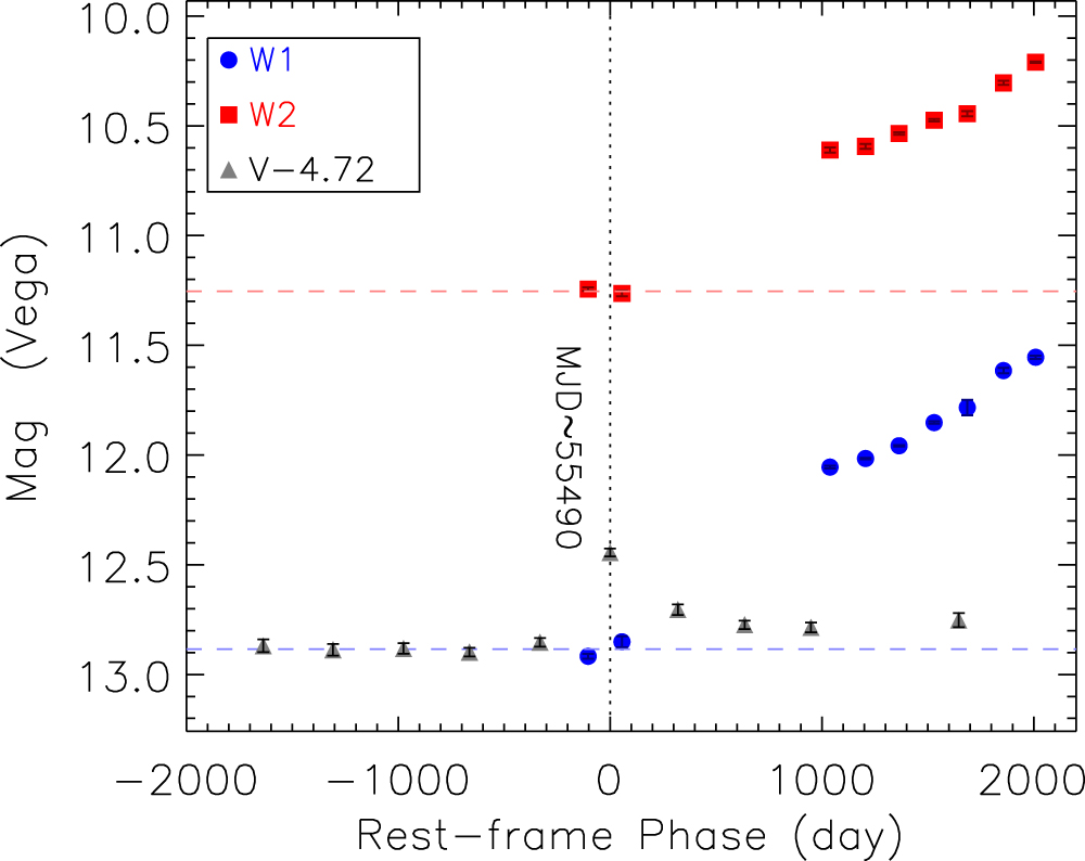
Optical (black triangles) and infrared (blue circles and red squares) observations of F01004–2237. Day 0 marks the day the optical emission peaked. The infrared emission rises steadily through the end of the data. [Dou et al. 2017]

Tidal disruption events occur when a star passes within the tidal radius of a supermassive black hole. After tidal forces pull the star apart, much of the stellar matter falls onto the black hole, radiating briefly in X-ray, ultraviolet and optical as it accretes. This signature rise and gradual fall of emission has allowed us to detect dozens of tidal disruption events thus far.

One of the recently discovered candidate events is a little puzzling. Not only does the candidate in ultraluminous infrared galaxy F01004–2237 have an unusual host — most disruptions occur in galaxies that are no longer star-forming, in contrast to this one — but its optical light curve also shows an unusually long decay time.

Now mid-infrared observations of this event have been presented by a team of scientists led by Liming Dou (Guangzhou University and Department of Education, Guangdong Province, China), revealing why this disruption is behaving unusually.

dusty torus

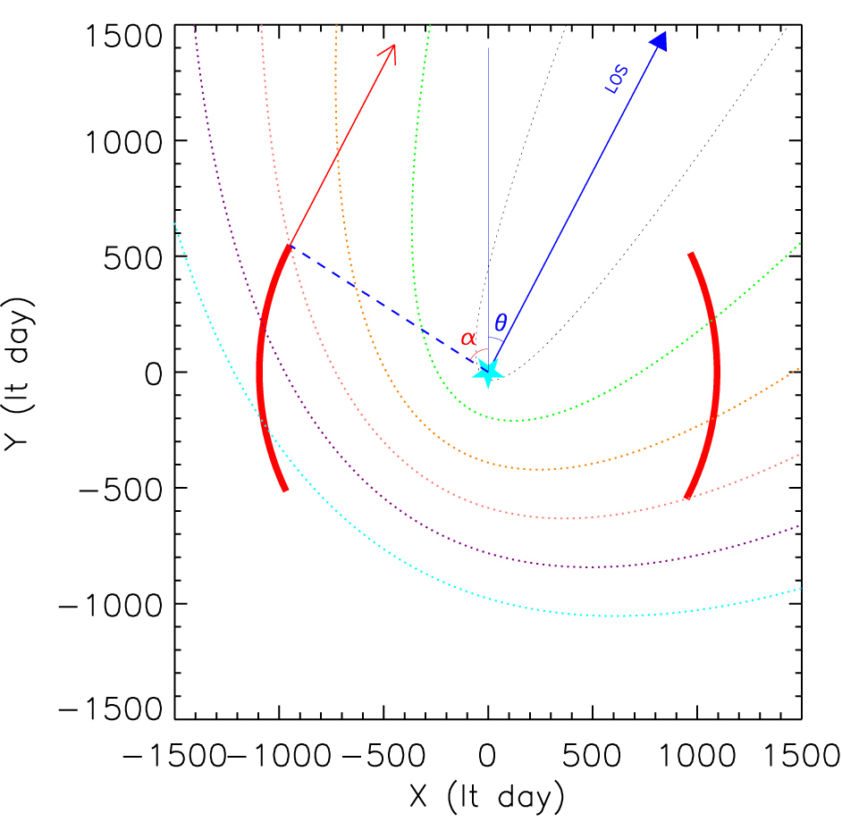
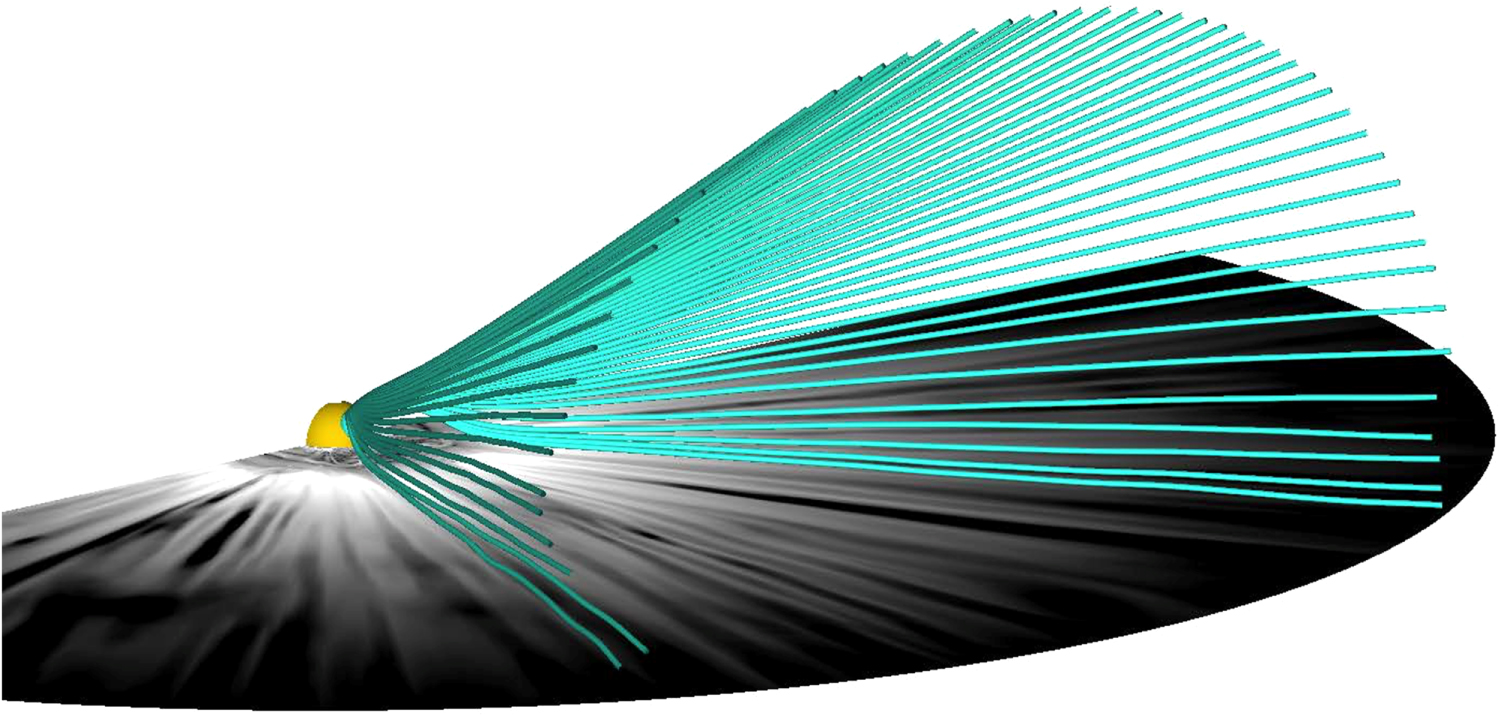
Schematic of a convex dusty ring (red bows) that absorbs UV photons and re-emits in the infrared. It simultaneously scatters UV and optical photons into our line of sight. The dashed lines illustrate the delays at lags of 60 days, 1, 2, 3, 4, and 5 years. [Adapted from Dou et al. 2017]

A Dusty Solution?

The optical flare from F01004–2237’s nucleus peaked in 2010, so Dou and collaborators obtained archival mid-infrared data from the WISE and NEOWISE missions from 2010 to 2016. The data show that the galaxy is quiescent in mid-infrared in 2010 — but in data from three years later, the infrared emission has significantly increased, and it continues to brighten steadily through the end of the data.

What’s going on? The supermassive black hole in the nucleus of F01004–2237 is likely shrouded by dust! The optical and ultraviolet radiation from the disruption is absorbed by the dust surrounding the black hole. This light is then reemitted as infrared radiation — which we see as a delayed echo of the flare, since the light had to travel out to the surrounding dust before being reemitted and traveling to us.

Modeling Echoes

Dust ring model

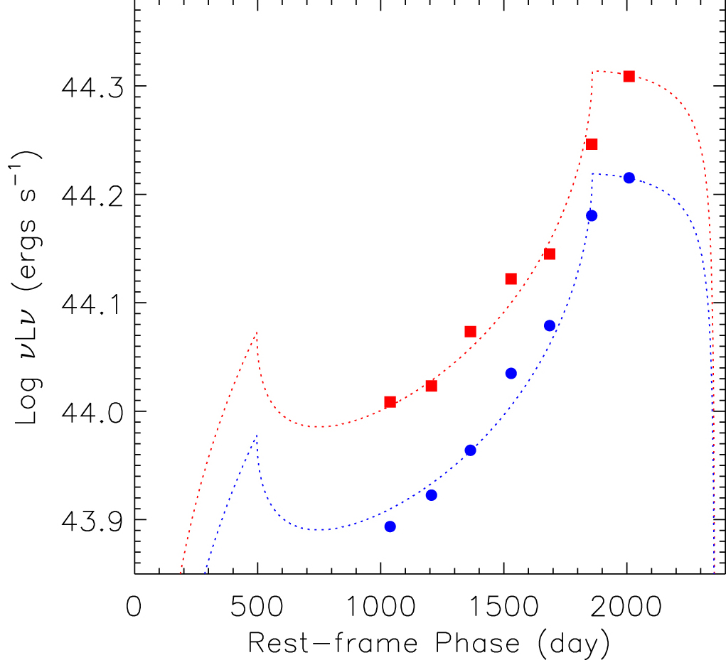
A fit of the data (points) to light curves (dashed lines) generated by one of the authors’ dust ring models. [Adapted from Dou et al. 2017]

Dou and collaborators show that the observations of F01004–2237 can be explained if the black hole is surrounded by a thick torus of at least 7 solar masses’ worth of dust, with a radius of at least 3 light-years. Such a large dust mass so close to the supermassive black hole implies that these dust grains can’t have been newly formed — so they must have already been there from the dusty torus of the galactic nucleus.

The authors point out that this dusty ring solves one of the mysteries of this disruption candidate: because the dust also scatters some of the optical light, this explains why the optical light curve didn’t decay as quickly as we’d expect.

Conveniently, the authors’ model of this event can be easily tested: it predicts a sharp decrease in the mid-infrared flux in the near future. Continued monitoring of F01004–2237 in mid-infrared channels should therefore soon be able to confirm our picture of this event. If we’re correct, these observations provide us with an excellent opportunity to learn about the environments around supermassive black holes.

Citation

Liming Dou et al 2017 ApJL 841 L8. doi:10.3847/2041-8213/aa7130

Photo of a complex stellar nebula studded with bright stars.

Homunculus Nebula

Hubble view of the Homunculus Nebula surrounding Eta Carinae [NASA Hubble Space Telescope/Jon Morse (University of Colorado)]

The incredibly luminous massive star Eta Carinae has long posed a challenge for astronomers to model. New observations are now in … so were our models correct?

Dramatic Target

The massive evolved star Eta Carinae, located ~7,500 light-years away in the constellation Carina, is the most luminous star in the Milky Way. Eta Carinae has a quite a reputation for drama: it has been very unstable in the past, exhibiting repeated eruptions that have created the spectacular Homunculus Nebula surrounding it. Its present-day wind has the highest mass-loss rate of any hot star we’ve observed.

Picture of Stellar Wind

Eta Carinae

Top panel: February 2017 observations of Eta Carinae in continuum (left) and H-alpha. Middle panel: the normalized radial profile for H-alpha and continuum emission. Bottom panel: the full width at half maximum for H-alpha and continuum emission of Eta Carinae. The H-alpha is about 2.5 to 3 milliarcseconds wider than the continuum. [Adapted from Wu et al. 2017]

In our goal to understand the late evolutionary phases of very massive stars, we’ve developed radiative-transfer models to explain the behavior of Eta Carinae. One of the most well-known models, developed by John Hillier and collaborators in 2001, describes Eta Carinae’s mass loss via stellar winds. With the right observations, this model is testable, since it predicts observable locations for different types of emission. In particular, one prediction of the Hillier et al. model is that the dense, ionized winds surrounding the star should emit in H-alpha at distances between 6 and 60 AU, with a peak around 20 AU.

This nicely testable hypothesis is rendered less convenient by the fact that it’s hard to get resolved images of Eta Carinae’s H-alpha emission. Its distance from us — and the fact that it’s shrouded in the complex nebula it created — have thus far prevented us from resolving the H-alpha emission from this star. Now, however, a team of scientists from Steward Observatory, University of Arizona have changed this.

Confirming the Model

Led by Ya-Lin Wu, the team obtained diffraction-limited images of Eta Carinae using the Magellan adaptive optics system. The observations, made in both H-alpha and continuum, show that the H-alpha emitting region is significantly wider than the continuum emitting region, as predicted by the model. In fact, the measured emission implies that the H-alpha line-forming region may have a characteristic emitting radius of ~25–30 AU — in very good agreement with the Hillier et al. stellar-wind model.

This confirmation is strong support of the physical wind parameters estimated for Eta Carinae in the model, like the mass-loss rate of 10^-3 solar masses per year. These parameters are enormously helpful as we attempt to understand the physics of strong stellar-wind mass loss and the late evolutionary phases of very massive stars.

Citation

Ya-Lin Wu et al 2017 ApJL 841 L7. doi:10.3847/2041-8213/aa70ed

ASKAP

A new telescope, the Australian Square Kilometre Array Pathfinder (ASKAP), has joined the search for energetic and elusive fast radio bursts. And in just a few days of looking, it’s already had success!

Elusive Transients

The Parkes radio telescope, which has detected all but five of the fast radio bursts published to date, has a very narrow field of view. [CSIRO]

Fast radio bursts are mysterious millisecond-duration radio pulses that were first discovered around a decade ago. Since that time — particularly in recent years — we’ve made some progress toward the goal of localizing them. We’re now fairly convinced that fast radio bursts come from outside of the galaxy, and yet they’re enormously bright — orders of magnitude more luminous than any pulse seen from the Milky Way.

Better identification of where these mysterious bursts come from would help us to determine what they are. But so far, we’ve discovered only around 30 such bursts, despite the fact that they’re estimated to occur at a rate of ~3,000 events per day across the whole sky.

Why are they so hard to find? Due to their short duration, effective detection would require instantaneous coverage of a very large fraction of the sky. The Parkes radio telescope — which has detected all but five of the fast radio bursts published to date — has a field of view spanning less than a square degree, significantly limiting our ability to rapidly survey for these transients.

FRB 170107

FRB 170107’s band-averaged pulse (top) and dynamic spectrum (bottom). [Bannister et al. 2017]

A New Array in Town

A new player is now on the scene, however, and it’s already had huge success. ASKAP is a wide-field radio telescope made up of an array of 12-meter antennas. Using phased-array-feed technology, ASKAP is able to instantaneously observe an effective area of 160 square degrees — an enormous field compared to Parkes’ 0.6 square degrees! This capability significantly increases our chances of being able to detect fast radio bursts.

In a new study led by Keith Bannister (Australia Telescope National Facility, CSIRO Astronomy and Space Science), a team of scientists presents results from ASKAP’s first 3.4-day pilot survey. Bannister and collaborators announce that in this brief time, ASKAP has already detected a fast radio burst: FRB 170107, an especially luminous, ~2 millisecond burst that confirms the presence of an ultra-bright population of fast radio bursts.

Looking to the Future

Localization of FRB 170107

Localization of FRB 170107. [Adapted from Bannister et al. 2017]

Using the multiple bands of ASKAP, the authors were able to constrain the position of FRB 170107 to a region just 8’ x 8’ in size. No known field galaxies exist in that region, so we’re still not sure exactly where it came from, but this localization is already a significant achievement.

The discovery and characterization of a burst already after such a short initial campaign suggests that ASKAP will become a very powerful tool for detecting fast radio bursts — including some of the rarest bursts, ultra-bright ones like FRB 170107. We finally appear to be poised to resolve some of the mysteries of this population of transients.

Citation

K. W. Bannister et al 2017 ApJL 841 L12. doi:10.3847/2041-8213/aa71ff

white dwarf

New Kepler observations of a pulsating white dwarf have revealed clues about the rotation of intermediate-mass stars.

Learning About Progenitors

Stars weighing in at under ~8 solar masses generally end their lives as slowly cooling white dwarfs. By studying the rotation of white dwarfs, therefore, we are able to learn about the final stages of angular momentum evolution in these progenitor stars.

Most isolated field white dwarfs cluster in mass around 0.62 solar masses, which corresponds to a progenitor mass of around 2.2 solar masses. This abundance means that we’ve already learned a good deal about the final rotation of low-mass (1–3 solar-mass) stars. Our knowledge about the angular momentum of intermediate-mass (3–8 solar-mass) stars, on the other hand, remains fairly limited.

Fourier transform of the pulsations from SDSSJ0837+1856. The six frequencies of stellar variability, marked with red dots, reveal a rotation period of 1.13 hours. [Hermes et al. 2017]

Record-Breaking Find

A newly discovered white dwarf, SDSSJ0837+1856, is now helping to shed light on this mass range. SDSSJ0837+1856 appears to be unusually massive: it’s measured at 0.87 solar masses, which corresponds to a progenitor mass of roughly 4.0 solar masses. Determining the rotation of this white dwarf would therefore tell us about the final stages of angular momentum in an intermediate-mass star.

In a new study led by J.J. Hermes (Hubble Fellow at University of North Carolina, Chapel Hill), a team of scientists presents a series of measurements of SDSSJ0837+1856 that suggest it’s the highest-mass and fastest-rotating isolated pulsating white dwarf known.

rotation distribution

Histogram of rotation rates determined from the asteroseismology of pulsating white dwarfs (marked in red). SDSSJ0837+1856 (indicated in black) is more massive and rotates faster than any other known pulsating white dwarf. [Hermes et al. 2017]

Rotation from Pulsations

Why pulsating? In the absence of measurable spots and other surface features, the way we measure the rotation rate of a star is using asteroseismology. In this process, observations of a star’s tiny oscillations can reveal information about its internal structure and rotation.

Hermes and collaborators used Kepler K2 observations spanning nearly 75 days — in addition to ground-based follow-up and spectroscopy — to estimate the white dwarf’s rotation period based on its observed internal pulsations. The resulting rotation rate, 1.13 ± 0.02 hours, is the fastest rotation period ever measured for an isolated pulsating white dwarf.

Placing SDSSJ0837+1856 in the context of other white dwarfs with measured rotation periods, the authors argue that there seems to be a connection between the highest-mass white dwarfs and the fastest rotators. More observations of this kind will help us to determine whether this is a general trend that tells us something significant about the angular momentum evolution of intermediate-mass stars.

Citation

J. J. Hermes et al 2017 ApJL 841 L2. doi:10.3847/2041-8213/aa6ffc

TW Hya

Observations of the protoplanetary disks that surround young stars provide crucial information about the initial conditions for planet formation. In a recent study, a team of scientists has proposed a novel new approach for determining disk properties from observations.

Limitations to Direct Measurement

protoplanetary disk

Artist’s impression of a protoplanetary disk surrounding a young star. [ESO/L. Calçada]

The surface density of protoplanetary disks (i.e., how much mass is there and where is it concentrated?) can’t be measured directly, since most of the disk mass is in molecular hydrogen gas, which doesn’t readily emit.

Instead, disk surface densities are inferred by measuring other components of the disk, like dust or molecules like CO or HD, and then making assumptions about the molecular abundances or the dust-to-gas ratio in the disk. Disk surface density estimates are therefore heavily dependent upon the assumptions that went into them.

Now, a team of scientists led by Diana Powell (University of California Santa Cruz) has proposed a new technique in which observations of a disk in different wavelengths can be used to determine its surface density profile without the need for such assumptions.

dust lines

Schematic showing disk dust lines for three different particle sizes, s1 > s2 > s3. Particles of size s1 exist in the yellow region, so in observations at wavelength λobs s1, a disk the size of the yellow region will be seen. Particles of size s2 exist in the yellow and red region, so a disk will extend to the end of the red region for λobs s2. Particles of size s3 exist throughout the disk, so the full disk size will be seen for λobs s3. [Powell et al. 2017]

How Does It Work?

Particles in a protoplanetary disk collide and stick together, thereby growing over time. But particles are also removed from the outskirts of the disk by a process called drift. More massive particles are removed from closer in to the star, so average particle sizes get smaller the further from the star you move out in a disk. For this reason, the disk’s radial size appears to be different in different wavelengths: at long wavelengths (i.e., looking at large particles) a disk might only span 50 AU, whereas at smaller wavelengths (looking at small particles) the same disk may span 300 AU. These different outer edges are known as dust lines.

The model proposed by Powell and collaborators relies on the idea that at a dust line for a given particle size, the growth timescale and drift timescale for particles of that size are both equal to the age of the disk. Setting these theoretical timescales equal at dust lines and using the age of the disk (expected to be the same as the age of the star, which is measurable) makes it possible to calculate the surface density profile for the disk. In this way, the profile can be measured without the need for assumptions about abundances or dust-to-gas ratios.

dust surface density

Dust surface density calculated by authors for TW Hya (blue points), compared to the dust surface density previously estimated for the system using an assumed dust-to-gas ratio (black line). The authors’ measurements are systematically lower. [Powell et al. 2017]

Testing the Approach

The team tested their technique on the disk TW Hya, finding a surface density profile that’s in agreement with lower limits set from measurements of the HD gas in the disk. Powell and collaborators then describe a series of observational tests of their technique that, when applied to a larger set of protoplanetary disks from future ALMA observations, will hopefully confirm the validity of their approach.

If this new method of measuring disk surface density profiles indeed proves successful, it could have an enormous impact on the field, making it much easier to learn about the evolution of protoplanetary disks and the planets forming within them.

Citation

Diana Powell et al 2017 ApJ 840 93. doi:10.3847/1538-4357/aa6d7c

the Sirius system

Sometimes important astronomical advances require the newest and fanciest observatories and technologies — but sometimes they just require decades of work and a lot of patience. Patience is finally paying off for a team of scientists who have been observing the Sirius star system for nearly 20 years.

Sirius observations

Historical (black, blue and green) and Hubble (red) observations of the relative orbit of Sirius B around Sirius A. [Adapted from Bond et al. 2017]

Bright Neighbors

Located a mere 8.5 light-years away, the Sirius system consists of the main-sequence star Sirius A and its white-dwarf companion Sirius B. Sirius A is the brightest star in our sky, and Sirius B is the brightest and nearest white dwarf we’ve observed. The unusual proximity and brightness of these stars make them excellent targets for learning about stellar and white-dwarf astrophysics.

In order to interpret our observations, however, we first need to pin down the basic information about these stars. In particular, we want to measure the precise masses and orbital elements for the system — but because the stars orbit each other only once every ~50 years, these properties take time to measure well!

Toward this end, a team of scientists began an observing campaign in 2001 to regularly image the Sirius system using the Hubble Space Telescope. Now, 16 years later, they have enough data to make precise statements about the system.

Precision Measurements at Last

In a recent publication led by Howard Bond (Pennsylvania State University and Space Telescope Science Institute), the team details nearly two decades of precise photometric and astrometric measurements using Hubble. In addition, they supplemented these data by dredging through 150 years’ worth of historical observations of Sirius and critically analyzing 2,300 of these as well.

white-dwarf theory

Comparisons of white-dwarf theory with the observed parameters of Sirius B, both on the H-R diagram (top) and in a mass-radius plot of cooling white dwarfs (bottom). Sirius B’s measured parameters matches the theoretical models very well. [Bond et al. 2017]

The result? Bond and collaborators were able to make very precise measurements of the masses of Sirius A and Sirius B — 2.063 ± 0.023 and 1.018 ± 0.011 solar masses, respectively — and of their orbital elements. They find that the position of Sirius B on the Hertzsprung-Russell diagram is beautifully consistent with models based on cooling white dwarfs of Sirius B’s measured mass. Similarly, stellar models of Sirius A are nicely consistent with Bond and collaborators’ measurements if the star has a slightly low metallicity of ~85% that of the Sun.

The high-precision measurements also allowed the authors rule out the possibility of a third body in the system — an idea that’s been tossed around for decades — unless the third body is smaller than 15–25 Jupiter masses.

Bond and collaborators enumerate some open puzzles of the Sirius system, such as like conflicting signs that the two stars might have interacted, long ago. Though these puzzles remain unresolved, the painstaking decades of observations of Sirius have already revealed much about the system and improved our understanding of stellar evolution. What’s more, these measurements give us an ideal launching point for future studies of these two objects. In the case of the Sirius system, patience has definitely paid off.

Citation

Howard E. Bond et al 2017 ApJ 840 70. doi:10.3847/1538-4357/aa6af8

black hole binaries

The recent successes of the Laser Interferometer Gravitational-Wave Observatory (LIGO) has raised hopes that several long-standing questions in black-hole physics will soon be answerable. Besides revealing how the black-hole binary pairs are built, could detections with LIGO also reveal how the black holes themselves form?

Isolation or Hierarchy

The first detection of gravitational waves, GW150914, was surprising for a number of reasons. One unexpected result was the mass of the two black holes that LIGO saw merging: they were a whopping 29 and 36 solar masses.

hierarchical merger schematic

On the left of this schematic, two first-generation (direct-collapse) black holes form a merging binary. The right illustrates a second-generation hierarchical merger: each black hole in the final merging binary was formed by the merger of two smaller black holes. [Adapted from Gerosa et al., a simultaneously published paper that also explores the problem of hierarchical mergers and reaches similar conclusions]

How do black holes of this size form? One possibility is that they form in isolation from the collapse of a single massive star. In an alternative model, they are created through the hierarchical merger of smaller black holes, gradually building up to the size we observed.

A team of scientists led by Maya Fishbach (University of Chicago) suggests that we may soon be able to tell whether or not black holes observed by LIGO formed hierarchically. Fishbach and collaborators argue that hierarchical formation leaves a distinctive signature on the spins of the final black holes — and that as soon as we have enough merger detections from LIGO, we can use spin measurements to statistically determine if LIGO black holes were formed hierarchically.

Spins from Major Mergers

When two black holes merge, both their original spins and the angular momentum of the pair contribute to the spin of the final black hole that results. Fishbach and collaborators calculate the expected distribution of these final spins assuming that all the hierarchical mergers are so-called “major mergers” — i.e., the smaller black hole of the pair is at least 70% of the mass of the larger one.

spin distribution

Distribution of spins for 4th-generation mergers, with two different mass ratios (= 0.7 and = 1) and initial first-generation spins (non-spinning and maximally spinning). [Fishbach et al. 2017]

The authors find that hierarchical major mergers result in a distribution of spins with a distinctive shape, peaking at a spin of a ~ 0.7 with relatively low contribution from spins below a ~ 0.5. Intriguingly, this distribution is universal — if you include several generations of mergers, the resulting spin distribution converges to the same shape every time. This is true regardless of the details of the hierarchical merger scenario, like the exact black hole mass ratio (as long as only major mergers occur) or the initial spin distributions.

Testing the Model

What does this tell us? Since the hierarchical merger model predicts a very specific distribution of spins for the black holes detected by LIGO, we can compare future LIGO detections to see if they’re consistent with this model.

The authors calculate the statistics to show that after order ~100 LIGO detections, we should be able to tell whether these black holes are consistent with a hierarchical merger formation model or not. With luck, this could mean that we will have solved this mystery within a few years of advanced LIGO operations!

Citation

Maya Fishbach et al 2017 ApJL 840 L24. doi:10.3847/2041-8213/aa7045

CubeSat

Major space-based observatories are imperative in astronomy, but they take a long time to plan, build, and launch — and they aren’t cheap. A new study examines an interesting compromise: a low-cost, space-based gamma-ray detector that we could use while we wait for the next big observatory to launch.

gamma-ray observatories

Coverage and sensitivity of past and future missions for the X-ray to gamma-ray energy range (click for a better look!). The only past mission to explore the 1 MeV region was COMPTEL, on board CGRO. e-ASTROGAM is a proposed future space mission that would explore this range. [Lucchetta et al. 2017]

A Gap in Coverage

In the last few decades, we’ve significantly expanded our X-ray and gamma-ray view of the sky. One part of the electromagnetic spectrum remains poorly explored, however: the approximate transition point between X-rays and gamma rays near 1 MeV.

Space-based gamma-ray telescopes have been proposed for the future to better explore this energy range. But these major observatories have costs of around half a billion Euros and will take roughly a decade to build and launch. Is there a way to get eyes on this energy range sooner?

Scaling Down with CubeSat

A team of scientists led by Giulio Lucchetta (University of Padova and INFN Padova, Italy) has proposed an intriguing solution for the more immediate future: a nano-satellite telescope based on the CubeSat standard.

proposed detector

Structure of the proposed gamma-ray detector, in a 2U CubeSat design. [Lucchetta et al. 2017]

A CubeSat is a miniaturized satellite design that can be easily deployed in space, either from the International Space Station or by hitching a ride as a secondary payload on a large rocket. The size of a CubeSat is a standardized unit of measurement: a single CubeSat unit, or 1U, is a mere 10x10x10 cm and a maximum of 1.33 kg in weight.

The gamma-ray telescope proposed by Lucchetta and collaborators would use a 2U standard for the instrument, so the instrument would be only 10x10x20 cm in size! The design for the telescope as a whole — including the on-board electronics and flight system — would likely require a 4U model.

The team’s proposed nanoscale observatory would be capable of detecting gamma rays from 100 keV up to a few MeV. In comparison to the major space-based observatories, this project would be very low-cost, at only half a million Euros — and such a telescope could go from build to launch in about a year.

Evaluating Performance

estimated sensitivity

Estimated sensitivity of the proposed nanoscale satellite telescope (for tracked, untracked, and pair production events) compared to that of COMPTEL. [Lucchetta et al. 2017]

Cheaper and faster is great, but how would this project do in terms of quality? The authors performed simulations to examine the scientific performance of the proposed detector, evaluating its effective area, energy resolution, and angular resolution. Luchetta and collaborators show that while the scientific performance would be well below that expected for large future missions, it would likely be on par with the last detector to observe this region — COMPTEL, on board the Compton Gamma Ray Observatory.

It seems that a nanoscale satellite like this one would helpfully cover the gap around 1 MeV and allow us to learn more about low-energy gamma rays while we wait for large future missions to launch. As an additional benefit, such a project could serve as a pathfinder mission to test technologies and algorithms to be used in larger missions in the future.

Citation

Giulio Lucchetta et al 2017 AJ 153 237. doi:10.3847/1538-3881/aa6a1b

Plasma from the Sun known as the slow solar wind has been observed far away from where scientists thought it was produced. Now new simulations may have resolved the puzzle of where the slow solar wind comes from and how it escapes the Sun to travel through our solar system.

An Origin Puzzle

coronal hole

A full view of a coronal hole (dark portion) from SDO. The edges of the coronal hole mark the boundary between open and closed magnetic field lines. [SDO; adapted from Higginson et al. 2017]

The Sun’s atmosphere, known as the corona, is divided into two types of regions based on the behavior of magnetic field lines. In closed-field regions, the magnetic field is firmly anchored in the photosphere at both ends of field lines, so traveling plasma is confined to coronal loops and must return to the Sun’s surface. In open-field regions, only one end of each magnetic field line is anchored in the photosphere, so plasma is able to stream from the Sun’s surface out into the solar system.

This second type of region — known as a coronal hole — is thought to be the origin of fast-moving plasma measured in our solar system and known as the fast solar wind. But we also observe a slow solar wind: plasma that moves at speeds of less than 500 km/s.

The slow solar wind presents a conundrum. Its observational properties strongly suggest it originates in the hot, closed corona rather than the cooler, open regions. But if the slow solar wind plasma originates in closed-field regions of the Sun’s atmosphere, then how does it escape from the Sun?

Slow Wind from Closed Fields

A team of scientists led by Aleida Higginson (University of Michigan) has now used high-resolution, three-dimensional magnetohydrodynamic simulations to show how the slow solar wind can be generated from plasma that starts out in closed-field parts of the Sun.

heliospheric arc

A simulated heliospheric arc, composed of open magnetic field lines. [Higginson et al. 2017]

Motions on the Sun’s surface near the boundary between open and closed-field regions — the boundary that marks the edges of coronal holes and extends outward as the heliospheric current sheet — are caused by supergranule-like convective flows. These motions drive magnetic reconnection that funnel plasma from the closed-field region onto enormous arcs that extend far away from the heliospheric current sheet, spanning tens of degrees in latitude and longitude.

The simulations by Higginson and collaborators demonstrate that closed-field plasma from coronal-hole boundaries can be successfully channeled into the solar system. Due to the geometry and dynamics of the coronal holes, the plasma can travel far from the heliospheric current sheet, resulting in a slow solar wind of closed-field plasma consistent with our observations. These simulations therefore suggest a process that resolves the long-standing puzzle of the slow solar wind.

Bonus

Check out the animation below, made from the results of the team’s simulations. This video shows the location of a forming heliospheric arc at a distance of 12 solar radii. The arc forms as magnetic field lines at the boundary of a coronal hole change from closed to open, allowing closed-field flux to escape along them.

Citation

A. K. Higginson et al 2017 ApJL 840 L10. doi:10.3847/2041-8213/aa6d72

full view of elliptical

MUSE fields of view

MUSE fields of view (1′ × 1′ for each square) are superimposed on a pseudo-color image of the elliptical galaxy in Abell 2670. The blue blobs lie in the opposite direction to the galactic center. [Sheen et al. 2017]

An elliptical galaxy in the cluster Abell 2670 has been discovered with some unexpected features. What conditions led to this galaxy’s unusual morphology?

Unexpected Jellyfish

We often see galaxies that have been disrupted or reshaped due to their motion within a cluster — but these are usually late-type galaxies like our own. Such gas-rich galaxies are distorted by ram pressure as they fall into the cluster center, growing long tails of stripped gas and young stars that earn them the name “jellyfish galaxies”.

But early-type, elliptical galaxies have long since used up or cleared out most of their gas, and they correspondingly form very few new stars. It’s therefore unsurprising that they’ve never before been spotted to have jellyfish-like features.

blobs

Panels a and b show zoomed-in observations of some of the star-forming blobs with tadpole-like morphology. Panel c shows a schematic illustration of how ram-pressure stripping causes this shape. [Adapted from Sheen et al. 2017]

New deep observations of an elliptical galaxy in the cluster Abell 2670, however, have revealed some unexpected structures for an early-type galaxy. Led by Yun-Kyeong Sheen (Korea Astronomy and Space Science Institute), a team of scientists now reports on the optical and spectroscopic observations of this galaxy, made with the MUSE instrument on the Very Large Telescope in Chile.

Tadpole Blobs

These observations reveal a number of features, including starbursts at the galactic center, 80-parsec-long tails of ionized gas, disturbed halo features, and several blue star-forming blobs with tadpole-like morphology in the surrounding region. The blobs have stellar tails that point in the direction of motion of the galaxy (toward the cluster center) and streams of ionized gas that point in the opposite direction.

All of these features are signs that this galaxy is being ram-pressure stripped as it falls into the center of the cluster. The star-forming blobs, for example, are exhibiting classic ram-pressure-stripping behavior: as a galaxy falls into the cluster center, streams of ionized gas blow downwind, and stars (which don’t respond as easily to the force of the wind) are left behind in a stream pointing upwind.

Gas from a Merger?

late-type galaxy

An example of a tidal tail drawn out from a disrupted late-type galaxy. The disrupted galaxy in Abell 2670 is, in contrast, an early-type, elliptical galaxy that should be gas-poor. [H. Ford, JHU/M. Clampin, STScI/G. Hartig, STScI/G. Illingworth, UCO, Lick/ACS Science Team/ESA/NASA]

But if this is an elliptical galaxy, where did the gas come from for the tails and the galactic-center star formation? To rule out the obvious, the authors first check that this galaxy really is an early-type elliptical. The galaxy’s color (reddened), morphology (elliptical and no sign of a stellar disk), and stellar velocities (no sign of stellar rotation) all confirm this.

The authors therefore speculate that the galaxy recently underwent a “wet merger” — a merger with a companion galaxy that was gas-rich. Much of this gas was driven to the center of the elliptical galaxy in the merger, and it’s now responsible for the starbursts there.

We’ll hopefully be able to draw stronger conclusions about this unusual galaxy after additional investigation into the amount of gas it contains and the galaxy’s star formation rate. In the meantime, this stripped elliptical makes for an intriguing puzzle!

Citation

Yun-Kyeong Sheen et al 2017 ApJL 840 L7. doi:10.3847/2041-8213/aa6d79

1 94 95 96 97 98 118