In December, AAS Nova Editor Susanna Kohler had the opportunity to fly aboard the NASA/DLR Stratospheric Observatory for Infrared Astronomy (SOFIA) with the German Receiver for Astronomy at Terahertz Frequencies (GREAT) instrument. This week we’re taking a look at that flight, as well as some of the recent science the observatory produced and published in an ApJ Letters Focus Issue.
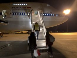
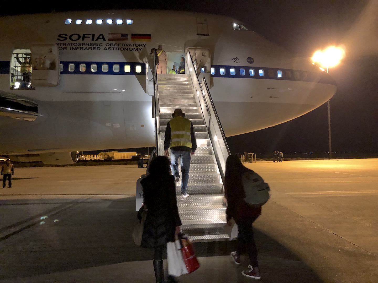
The SOFIA team and a handful of invited guests board the plane before a night in the stratosphere. [AAS Nova/S. Kohler]
It was 6 pm and I was boarding a plane for a 10-hour flight — but there were plenty of signs that this wasn’t your typical redeye.
For starters, I’d completed rigorous safety training earlier that day that included instructions on how to rappel down from the escape hatch of the cockpit.
Another sign was the catering (or lack thereof): no little bags of peanuts or lukewarm trays of airplane food. We each brought our own snacks, and we would be eating them cold — the microwave perched above the mini-fridge was off-limits tonight. The instrument currently mounted on the telescope was sensitive to potential leaked radiation from the microwave; no one wanted to be that guy whose nuked burrito ruined the night’s data.
My travel companions were another indicator that this was no normal flight: there were only 26 other people aboard, most of whom were dressed in flight jumpsuits adorned with mission patches. All of us were bundled up against the slow chill of the 60°F cabin and wearing communication headsets.
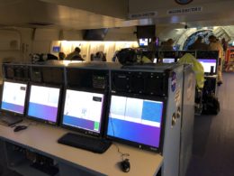
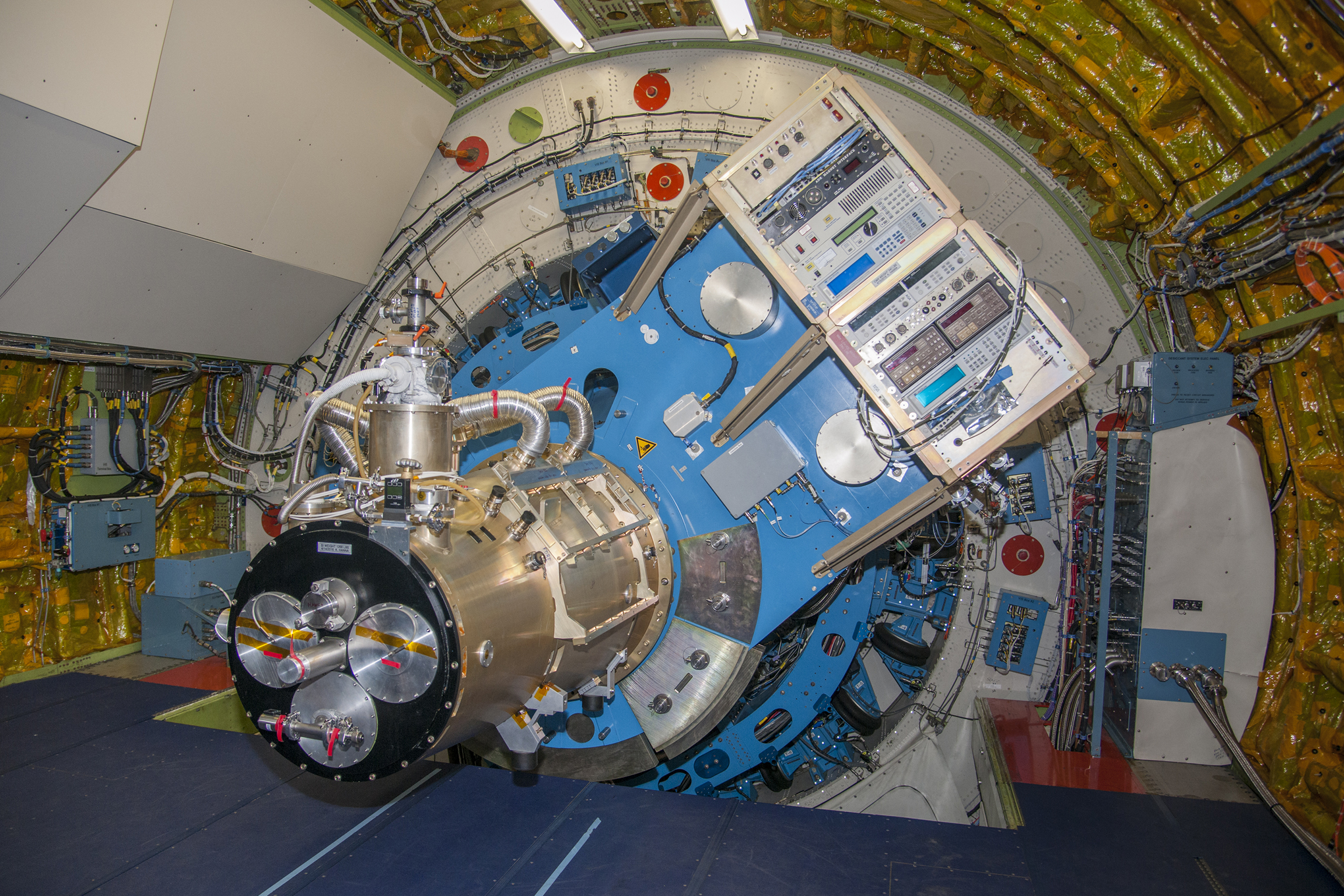
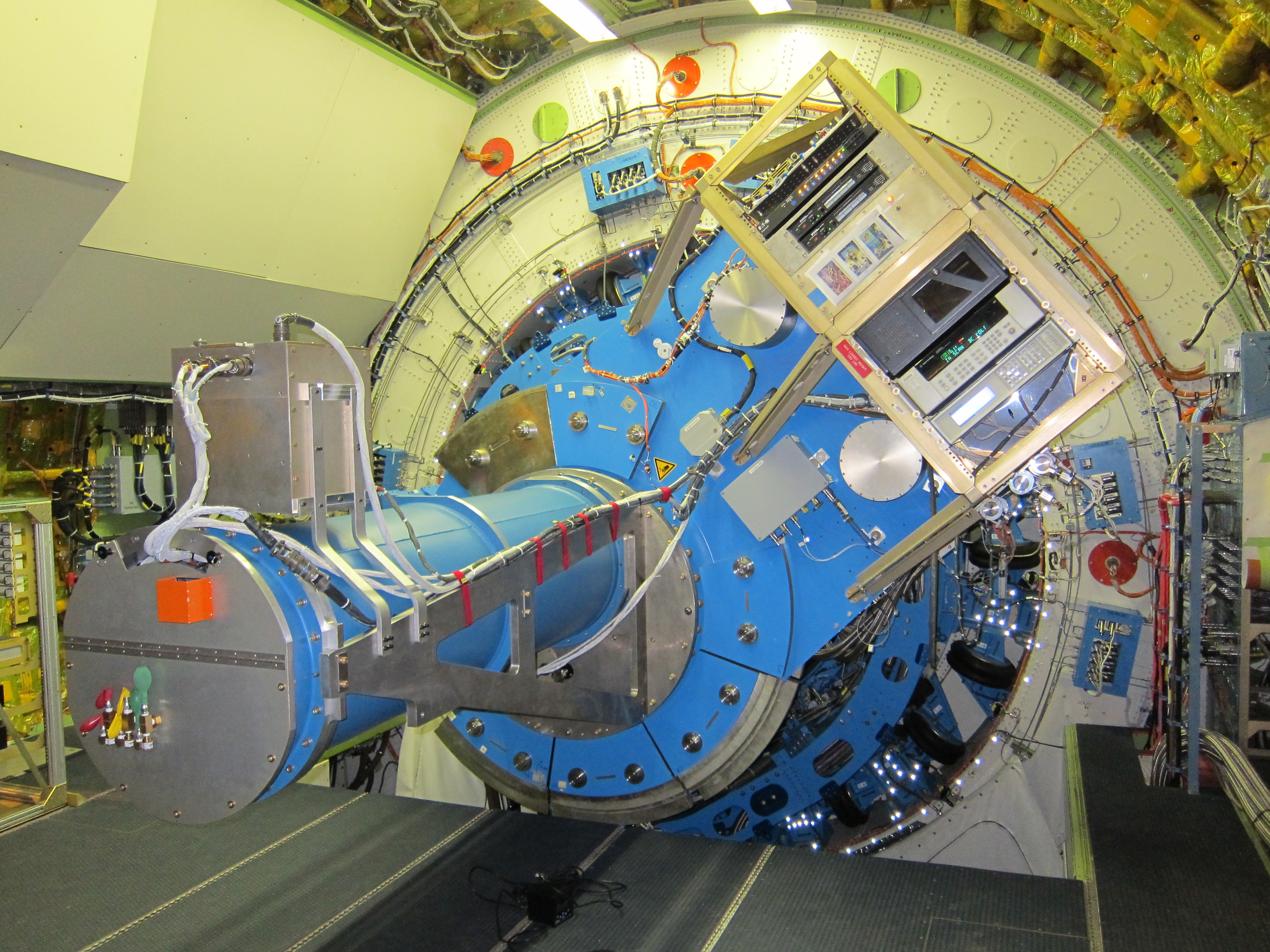
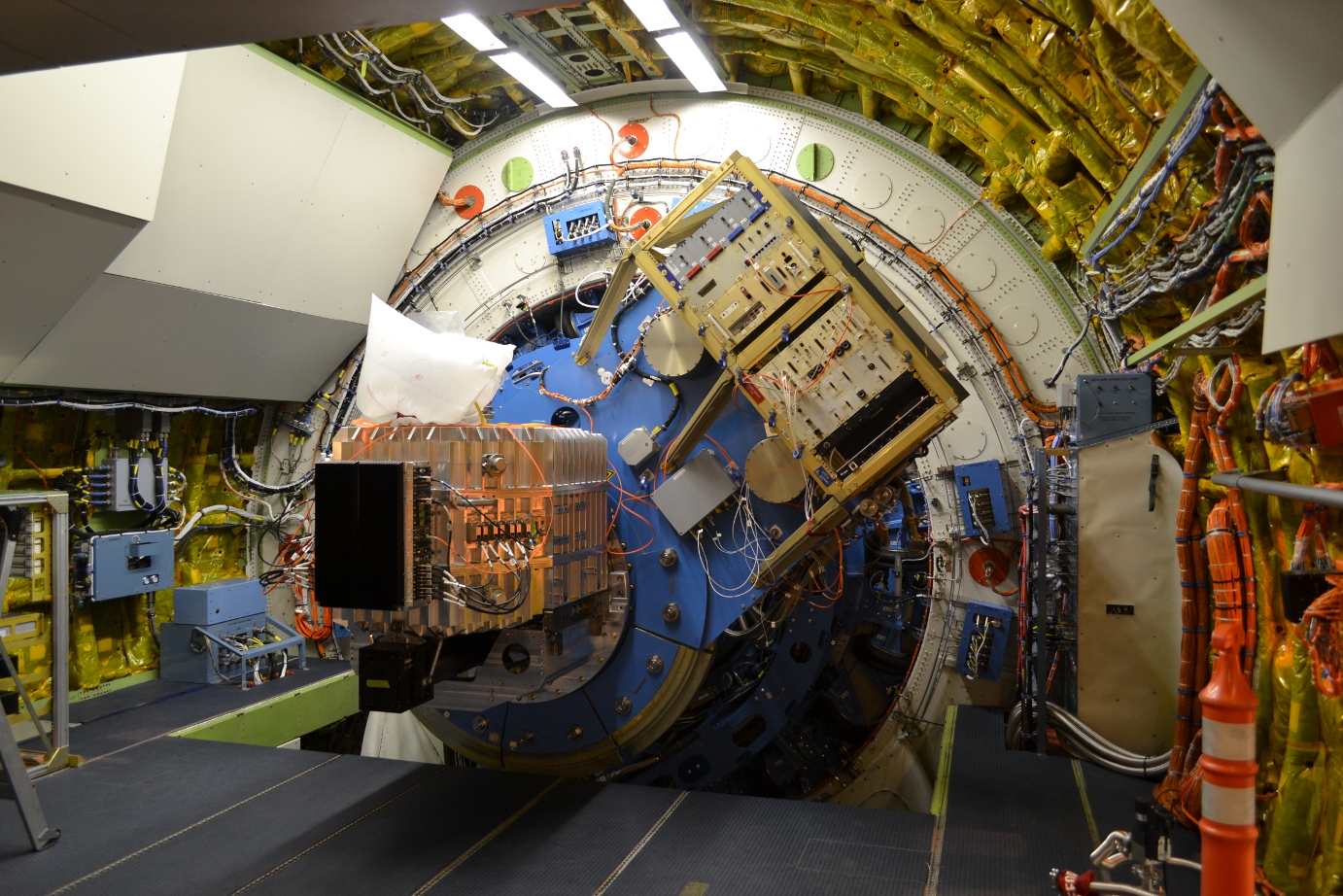
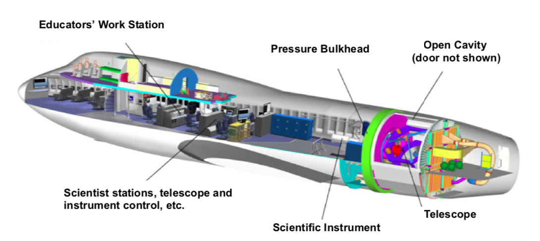
SOFIA’s cabin, facing the rear of the plane. The educator consoles in the foreground allow guests to follow along with the observations. The mission directors sit at the next set of consoles. At the rear of the plane is the solid bulkhead separating the telescope cavity; the GREAT instrument is visible just in front of this, mounted on the back of the telescope. [AAS Nova/S. Kohler]
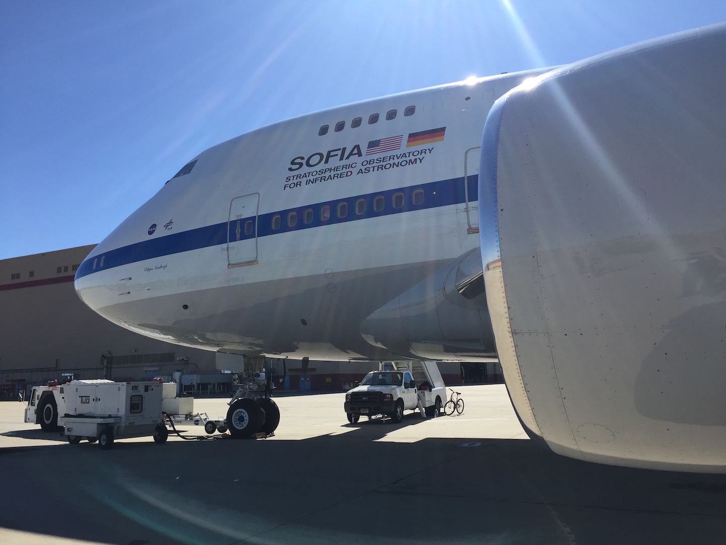
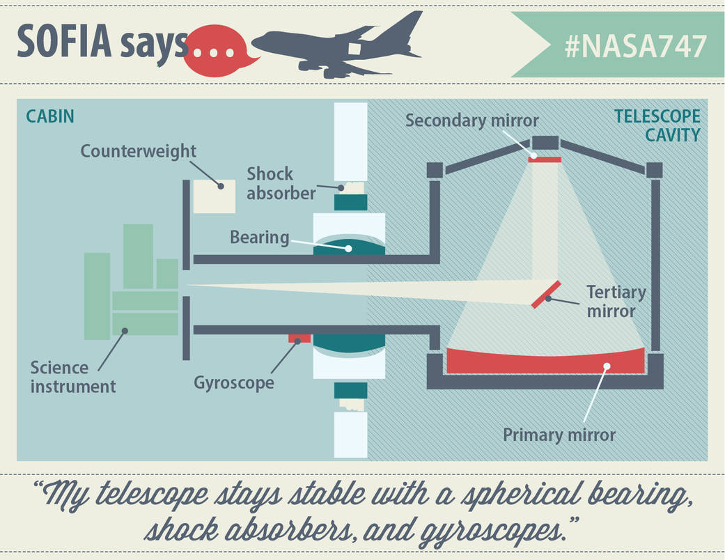
We were aboard SOFIA — the Stratospheric Observatory for Infrared Astronomy — and we were getting ready for a night of flying through the sky, doing infrared astronomy from the stratosphere.
Auspicious Beginnings
Takeoff was surprisingly quick: a short taxi and rapid climb into the air. The strangeness of the steep ascent was intensified by my seat: I’d been offered a spot at a console in front of a panel of computers, facing the tail of the plane. I’ve never taken off facing backwards before; I was grateful for the shoulder harness that kept me securely in my seat!
Onboard as an invited science writer, I had the great fortune of multiple guides on my flight; in addition to communication manager Nicholas Veronico, science outreach lead Randolf Klein flew with me that evening. As we listened in on our headsets to the chatter between the various team members, Randolf acted as my SOFIA translator, clarifying what was happening and what we could expect.
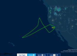
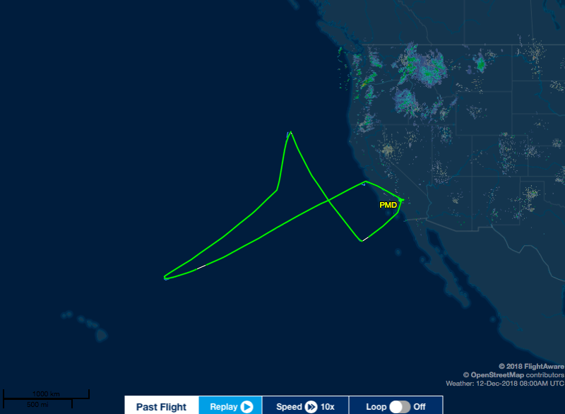
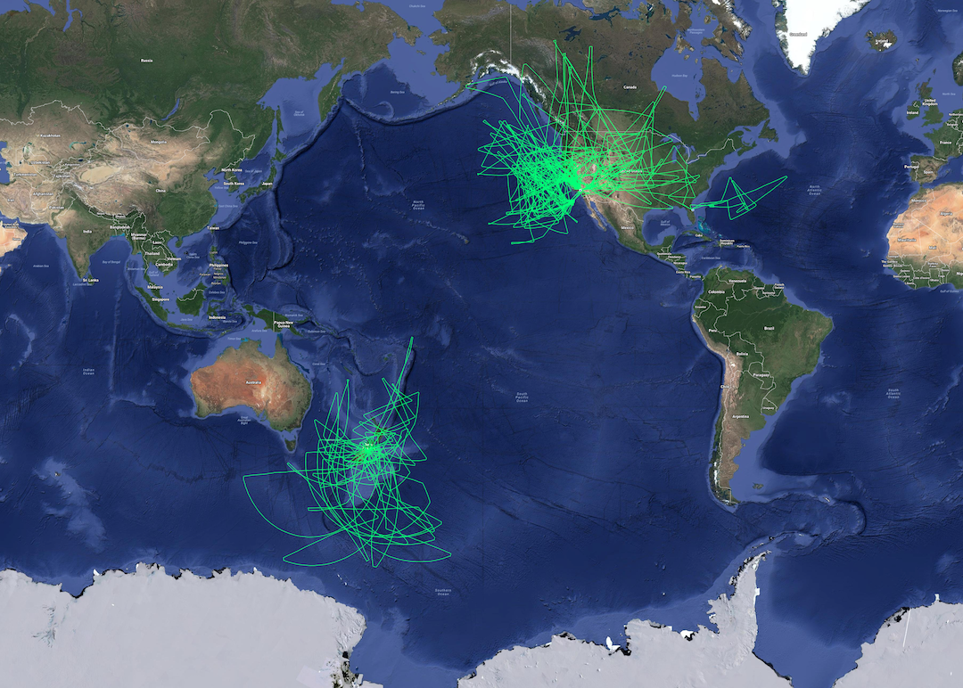
Screen capture from flightaware.com of our flight path for the night.
There’s Science to Be Done!
We would be observing with the German Receiver for Astronomy at Terahertz Frequencies (GREAT) instrument, and the goals for the night were clearly laid out. We’d begin with a short leg as we flew away from the coast and out over the Pacific, during which the door would open and the telescope would be initialized.
During our next, 130-minute leg, we would be roughly paralleling California’s coastline, heading as far north as the Oregon border. GREAT — a high-resolution spectrometer — had just been swapped onto SOFIA, so we would use this leg to point southwest at Mars, a known target that could be used to properly align the instrument for the remainder of its flights during this rotation.
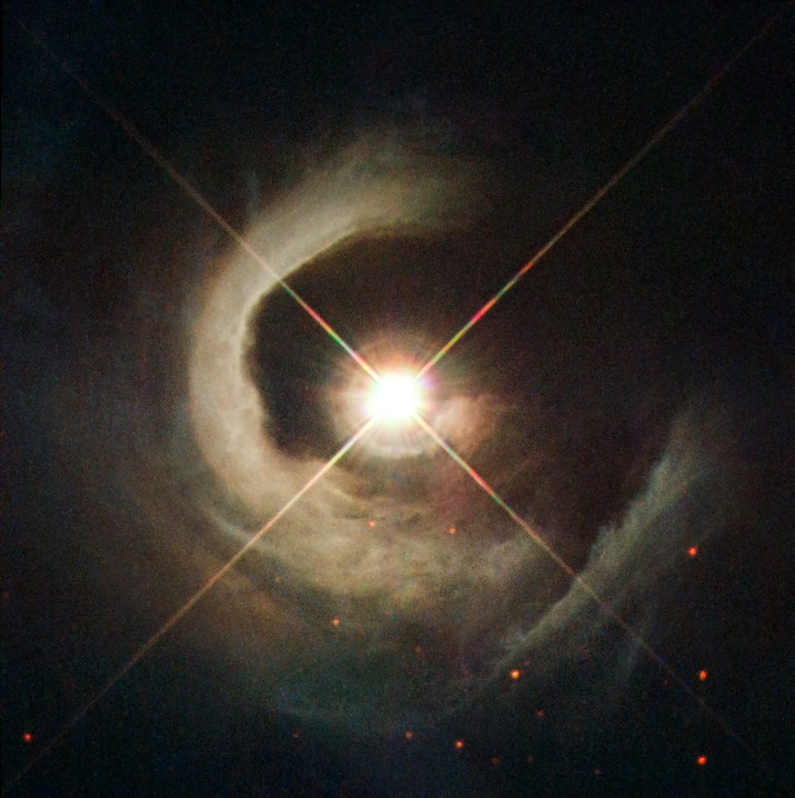
In the next leg, we’d turn southward and point the telescope toward the evolved star U Orionis. On this 37-minute segment, we’d capture spectra to study the physical processes responsible for exciting water masers — emission sources that work like naturally occurring lasers — in the star’s outer shells.

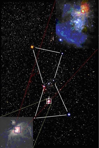
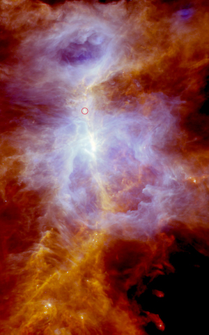
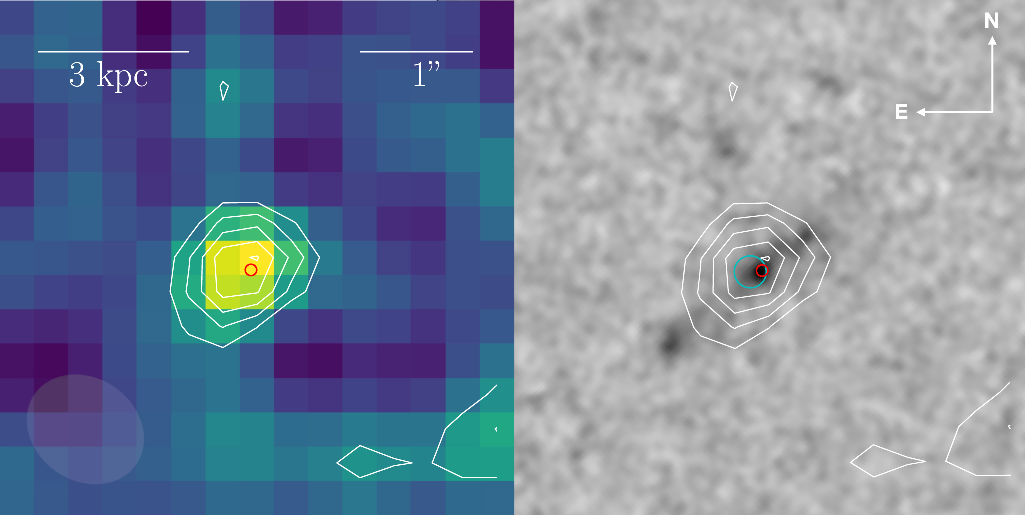
The Orion A star-forming region, as imaged by Herschel. OMC2 FIR4, the specific region we were exploring with SOFIA tonight, is circled in red. [ESA/Herschel/Ph. André, D. Polychroni, A. Roy, V. Könyves, N. Schneider]
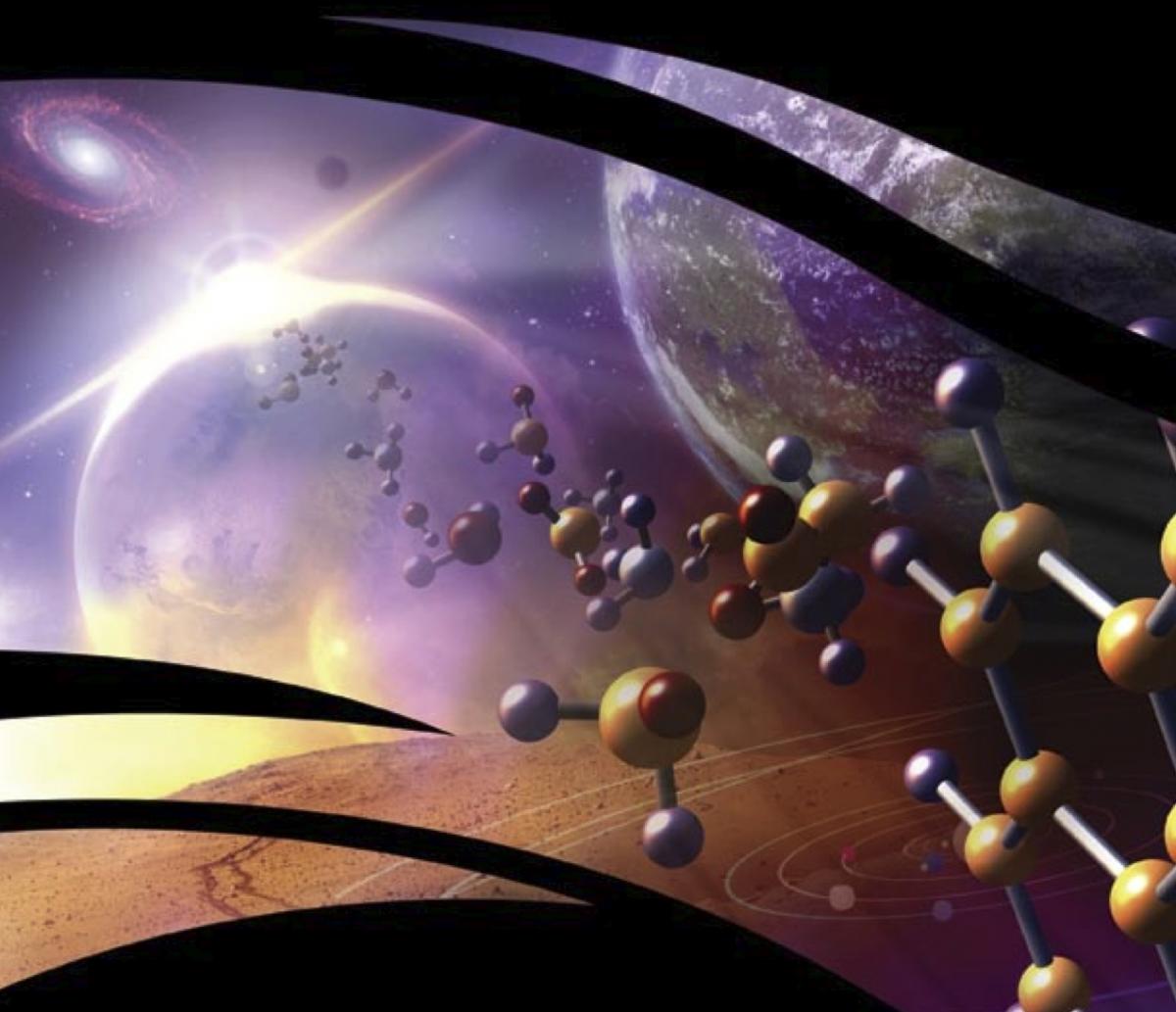
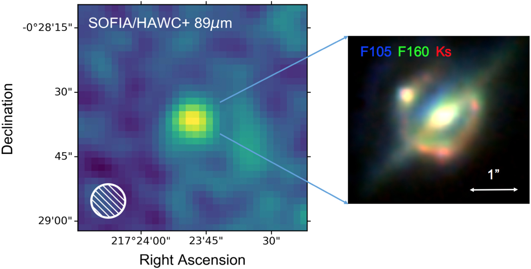
Next we would swing in the direction of Hawaii and fly roughly three-quarters of the way out to the islands, completing a 125-minute leg observing a specific molecule, deuterated hydroxyl (OD), in a stellar nursery in the Orion A molecular cloud. From these observations, scientists hope to explore the origins of some of the simplest molecules found in our universe.
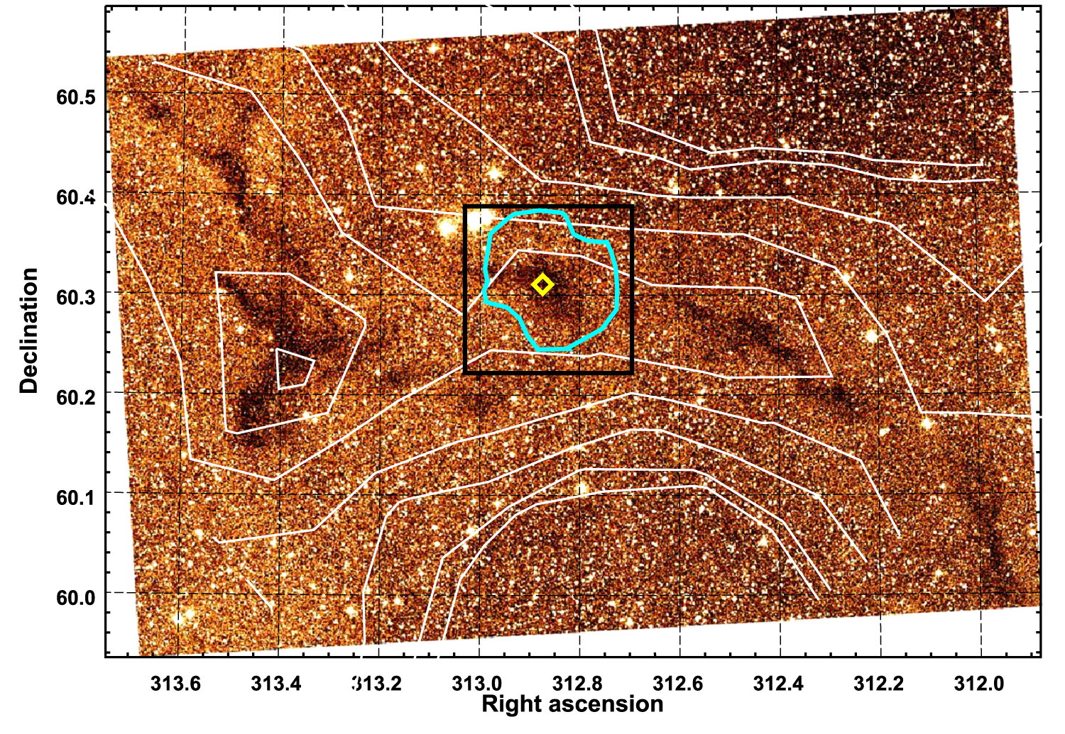
Lastly, we’d turn back to the northeast and fly a final long leg home, pointing at the W3 massive star-forming region in Cassiopeia to better understand the emission we see in the HII regions that surround young stars.
Suspense in the Stratosphere
The goals may have been clear, but astronomers know that observing never goes exactly as planned.
For us, the first challenge came early on: shortly into the telescope initialization leg, we hit sudden, strong turbulence. From the chatter in our headsets and the telescope’s view plotted on the console in front of me — which suddenly contained wildly swinging stars rather than the stable targets of moments before — it was clear that something had gone wrong.
Randolf explained: the turbulence had knocked the telescope into safe mode, and if the team couldn’t quickly reset the scope and complete the instrument alignment before our current leg ended, the entire night’s mission was at risk.
Thankfully, SOFIA’s team is used to handling challenges under time pressure. Before the leg was up, both the telescope and instrument were set up and aligned, and we all breathed a sigh of relief as the plane turned southwest onto our first science leg.
A Team Effort
Watching the data stream in on the screens in front of me that night was an exciting experience. Several of the GREAT team members were armed with laptops and were analyzing the data as fast as it arrived; since spectra can be hard to gauge by eye, real-time computer processing was a must to determine whether the team was getting what they needed.
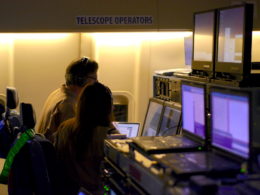
The telescope operators hard at work during our flight. [AAS Nova/S. Kohler]
Even more fascinating than seeing the data, however, was watching how the different subgroups of the SOFIA team worked together throughout the night to obtain the observations. The onboard team included three pilots, two mission directors, two telescope operators, and nearly a dozen scientists — both instrument and data specialists — associated with GREAT.
Constant adjustments were needed during the flight: if the pilots were notified of altitude constraints from the FAA, this would be relayed to the mission directors, who might modify the flight plan or observing times; if the scientists weren’t happy with the data they analyzed, they might make requests of the telescope operators or the instrument specialists. Meanwhile, the mission directors kept the team on track with regular announcements about how much time was left in each leg.
This complex stream of communication between groups took place over many radio channels and in multiple languages, and I found the apparent ease with which the team navigated it oddly beautiful and humbling.
Window into Our Universe
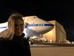
AAS Editor Susanna Kohler after a night flying aboard SOFIA. [AAS Nova/S. Kohler]
As the final observing leg wrapped up, I headed up to the flight deck for a rare opportunity to sit in a 747 cockpit during landing. Chatting with the three pilots — who had more than 300 SOFIA flights under their collective belts — I could tell that they enjoyed being a part of the team. Flying planes is pretty cool, but flying planes for science? That’s something else.
Our runway lights flicked on, guiding our way to a landing in the quiet California desert. As I looked up through the cockpit glass at the night sky, reflecting on my remarkable flight experience, one thing was clear: SOFIA is an extraordinary window into our universe.
*****

A successful flight! [AAS Nova/S. Kohler]
Check back tomorrow to learn about some of the recent science conducted with SOFIA.
Further Reading


