Features RSS

self-lensing

Though Kepler’s primary mission ended years ago, the resulting dataset remains a vast playground in which astronomers continue to discover new surprises in stellar light curves. The latest? Evidence of a white dwarf that defies all expectations.

Forming a Lightweight

ELM white dwarf

Artist’s impression of an extremely low-mass white dwarf (foreground) orbiting a more typical white dwarf (background). [CfA/David A. Aguilar]

White dwarfs come in a range of different sizes. A typical white dwarf might be around 0.6 solar mass and arise when an isolated star of perhaps a few times the mass of the Sun expands into a red giant, exhausts its fuel supply, and puffs off its outer layers, leaving behind its dead, dense core.

But some observed white dwarfs have much lower masses — say, between 0.15 and 0.3 solar mass. To produce such a small remnant mass, the mass of the initial progenitor star would also have to be very low. But this poses a problem: smaller stars take longer to evolve, so a star of such low mass would need longer than the age of the universe to exhaust its fuel supply!

Since isolated stellar evolution can’t explain extremely low-mass white dwarfs, astronomers have settled on another explanation: binary interactions. In this scenario, the close orbit of two stars in a binary results in material being stripped away from the progenitor star, accelerating its mass loss and allowing it to evolve into a very low-mass white dwarf.

So far, this explanation has fit our observations. But now, the discovery of a new low-mass white dwarf is challenging our understanding.

self lensing diagram

Example diagram of a different self-lensing binary system, KOI-3278. When the white dwarf passes between us and the primary star, gravitational magnification causes a brightening in the light curve that we detect. For KIC 8145411, we do not observe an occultation, because the light from the white dwarf is too faint to detect directly. [Eric Agol]

Self-Lensing Surprise

In a new publication, a team of scientists led by Kento Masuda (NASA Sagan Fellow at Princeton University) present the discovery of the binary system KIC 8145411 from Kepler data. This unique binary is one of only five known self-lensing systems: one object in the binary gravitationally lenses the light of the other as it passes in front once per orbit.

Masuda and collaborators use follow-up observations from the Fred Lawrence Whipple Observatory in Arizona and the Subaru telescope in Hawaii to pin down the properties of the system, confirming that we’re looking at a 0.2 solar-mass white dwarf orbiting a Sun-like star in an edge-on, eclipsing orbit.

But here’s the catch: KIC 8145411’s orbit is quite wide, at 1.28 AU (a period of ~450 days) — ten times too wide for the primary and the white-dwarf progenitor to have interacted in the way we’d expect. How, then, did this “impossible” white dwarf come to exist?

Tip of the Iceberg

white dwarfs in binaries

Masses of known white dwarfs in binaries and their orbital periods. The KIC 8145411 system is a clear outlier, having both a low mass and a very wide orbit. Click to enlarge. [Masuda et al. 2019]

Masuda and collaborators discuss a few proposed formation mechanisms — like interactions with a since-ejected or swallowed tertiary object — but none of them are especially satisfying.

So what’s next? The authors point out that we had only a 1 in 200 chance of detecting this particular system, due to its edge-on orientation — which likely means that KIC 8145411 is just the tip of the iceberg. Now that we know what we’re looking for, dedicated searches may turn up many more of these systems in the future — hopefully helping us to explain why this white dwarf is possible after all!

Citation

“Self-lensing Discovery of a 0.2 M White Dwarf in an Unusually Wide Orbit around a Sun-like Star,” Kento Masuda et al 2019 ApJL 881 L3. doi:10.3847/2041-8213/ab321b

black hole neutron star binary

There’s still a lot we don’t know about the internal structure and behavior of neutron stars, the compact remnants of giant, collapsed stars. Can the mergers of neutron stars with another type of exotic object, black holes, reveal important information?

Uncharted Remnants

gamma-ray bursts

Illustration of a short gamma-ray burst, which could be produced during the collision of a neutron star with a black hole. [ESO/A. Roquette]

Since neutron stars were first theorized, we’ve observed about 2,000 of them in the Milky Way and the Magellanic Clouds. Due to the exotic high-density conditions inside neutron stars, however, we still don’t well understand their interior structure and behavior.

A star’s internal properties are characterized by its “equation of state”. To better constrain the equation of state for neutron stars, we need accurate measurements of their masses and radii. But though we know that neutron stars are typically have the mass of a couple of Suns packed into a sphere of order 10 km in radius, it’s challenging to get precise enough radius measurements to constrain the equation of state for these dense, distant objects.

Can we do a better job of measuring neutron-star radii using future observations of merging neutron-star–black-hole binaries? A team of scientists led by Stefano Ascenzi (Tor Vergata University of Rome, INAF Rome Observatory, and Sapienza University of Rome, Italy) thinks the answer is yes — and in a new study, the team outlines how.

A Well-Marked Collision

It’s expected that the merger of a neutron star with a black hole would result in the destruction of the neutron star, the brief formation of a torus around the black hole as the neutron-star matter rains back down, and the rapid accretion of the torus.

This process would produce a pair of observable signals: 

  1. a gravitational-wave chirp from the merger, visible to detectors like the Laser Interferometer Gravitational-wave Observatory (LIGO) and its European counterpart Virgo, and
  2. a short gamma-ray burst (GRB) caused by the accretion of the torus.
equations of state

Example of how the various curves of mass vs. radius described by different neutron-star equations of state (colored curves) could be eliminated based on mass and radius measurements of a neutron star during a merger. In this test run, the authors’ injected neutron star properties are shown by the blue dot and the recovered properties are shown by the red dot. The red dashed lines show the 68% and 90% credible regions for the recovered properties — which, in this example, eliminate several of the possible equations of state. [Adapted from Ascenzi et al. 2019]

According to Ascenzi and collaborators, we can use these two signals in tandem to obtain information about the neutron star. Fitting the gravitational-wave signal of such a merger will reveal the neutron-star and black-hole masses, as well as the spin of the black hole. Measurements of the short GRB energy will tell us how much mass was in the torus that accreted onto the black hole.

The combination of this information allows us to infer the radius of the neutron star in the initial binary. Ascenzi and collaborators show that this method would let us estimate a neutron star radius to within 20% accuracy for a gravitational-wave detection with a signal-to-noise ratio of 10. For comparison, the signal-to-noise ratio for GW 170817, the first observed binary neutron star merger, was more than 30.

Looking for a New Type of Merger

How lucky do we have to get to observe a neutron-star–black-hole merger simultaneously in gravitational waves and electromagnetic radiation? Theory predicts these joint detections will perhaps occur at rates of 0.1 to 10 per year with current technology, and future telescopes and gravitational-wave detectors should increase our odds.

Here’s hoping these spectacular explosions will reveal more about neutron-star interiors soon!

Citation

“Constraining the Neutron Star Radius with Joint Gravitational-wave and Short Gamma- Ray Burst Observations of Neutron Star–Black Hole Coalescing Binaries,” Stefano Ascenzi et al 2019 ApJ 877 94. doi:10.3847/1538-4357/ab1b15

Beehive Cluster

Many people start to slow down as they age, and stars seem to be the same way. Astronomers measure how fast stars spin to determine their ages, but new measurements suggest that some stars may wind down more quickly than others.

Color-magnitude diagram

Color-magnitude diagram for globular cluster M55. Stars with masses higher than the turn-off point mass have lived long enough to evolve off the main sequence. [B.J. Mochejska, J. Kaluzny (CAMK), 1-m Swope Telescope]

Assigning Ages

It’s relatively straightforward to determine the age of a star that belongs to a cluster. The age of the cluster — and the stars that comprise it — is equal to the hydrogen-burning lifetime of the stars that are just about to swerve off the main sequence and balloon into red giants.

It’s much more challenging to measure the age of an isolated star. Astronomers rely on a method called gyrochronology — measuring a star’s age from the seemingly predictable slowdown of its rotation over time.

Stellar rotation periods appear to increase with the square root of the star’s age, but recent observations have hinted that that may not be true for all stars.

Evidence from Star Clusters

A team led by Jason Lee Curtis (Columbia University) studied F, G, and K stars to determine if the slowdown rate depends on mass. They used light curves from the Kepler spacecraft to measure the rotation periods of stars in NGC 6811, an open cluster in the constellation Cygnus. Curtis and collaborators used the observed rotation periods of the F and G stars in NGC 6811 to pinpoint the cluster’s age at 1.04 billion years.

Curtis et al. 2019 Fig. 5

Comparison of rotation periods for stars in NGC 6811 (blue, red, and cyan symbols) to models of Praesepe at 670 million and 1 billion years old (gray and black curves). The observed stellar rotation rates begin to diverge from the expected behavior around 5,400 K. [Curtis et al. 2019]

Next, they turned to a younger open cluster, Praesepe, which clocks in at around 670 million years old. Using a gyrochronology model derived from Praesepe’s observed stellar rotation periods, the authors artificially aged the cluster to 1 billion years old — the same age as NGC 6811. If all stars spin down the same way, the rotation rates of the artificially aged cluster should match those from NGC 6811.

Instead, although the rotation rates of the F and G stars from the two clusters matched neatly, NGC 6811’s lower-mass K stars were spinning faster than expected. In fact, they lined up almost perfectly with the K stars in the much younger cluster. In other words, while the F and G stars had slowed down with age, the K stars seemed to have not slowed down a bit in at least 330 million years.

Curtis et al. 2019 Fig. 7

Stellar ages derived from gyrochronology for NGC 6811 and the Hyades Cluster, compared to the 670-million-year-old Praesepe model. [Adapted from Curtis et al. 2019]

Why the Slow Pace?

One interpretation of this finding is that a star’s spin-down rate depends on its mass, with lower-mass stars winding down more slowly. However, the authors cautioned that it may not be that simple. Instead, they posited that stars experience a period during which their rotation rates don’t slow down — and lower-mass stars spend more time in this stalled spin-down state than higher-mass stars.

The authors aren’t sure what causes the stars to take a break from spinning down. They suggested that the stars either temporarily experience less magnetic braking or their outer layers gain angular momentum from their interiors.

Curtis and collaborators hope that studies of even older clusters, like 2.5-billion-year-old Ruprecht 147, will reveal at what point K dwarfs resume their usual spin-down and lead to a better understanding of how rotation rates can be used to determine the ages of stars.

Citation

“A Temporary Epoch of Stalled Spin-down for Low-mass Stars: Insights from NGC 6811 with Gaia and Kepler,” J. L. Curtis, M. A. Agüeros, S. T. Douglas, and S. Meibom 2019 ApJ 879 49. doi:10.3847/1538-4357/ab2393

atmospheric stripping

Can we use clues from the present to figure out how a planet has been blasted by the radiation of its host star in the past? According to a new study, it’s a definite possibility.

A History of Rotation and Radiation

rotation-period curves

Three example rotation-period curves show that stars can start with very different rotation rates and evolutionary tracks, but after 2 billion years, the tracks all converge. [Kubyshkina et al. 2019]

The history of a star’s radiation — its stellar flux evolution history — is important not just for what it tells us about the star, but also for the implications for nearby planets. Stars that emit large amounts of high-energy radiation early in their histories can wear away the atmospheres of fluffy, Neptune-like planets, leaving behind cores with thinner atmospheres like Earth’s or even no atmosphere at all.

How can we tell how much flux a star has historically emitted? This is tricky! We know that stars that rotate faster produce more high-energy radiation. But though stars are born with vastly different spin rates, they all lose angular momentum and spin down over time.

For a while, all these spin-down tracks are unique. But after about 2 billion years of slowing down, the tracks for stellar rotation evolution converge — if you’re looking at a star older than 2 billion years, you can no longer directly tell from its current properties how fast it rotated in the past, or how much flux it consequently emitted over its history.

But if a star has a sub-Neptune-sized planet in a close orbit? According to a new study led by Daria Kubyshkina (Austrian Academy of Sciences), we might then be able to make some inferences!

Clues from a Modern Atmosphere

For stars hosting close-in planets with hydrogen-dominated atmospheres, a bit of creative modeling of a planet’s atmospheric evolution can allow us to infer its host’s flux evolution history.

recovery of injected signal

Recovery of an injected signal in the authors’ analysis. In this example, the mass of the planet is assumed to be exactly known. The posterior distributions for the other parameters of the system (blue curves) well match the prior distributions of the input parameters (red curves). From top to bottom, the parameters are the stellar rotation period at 150 Myr, age of the system and present-time rotation period, and orbital separation and stellar mass. [Adapted from Kubyshkina et al. 2019]

The amount of hydrogen atmosphere a planet has left later in its life — which can be estimated from the planet’s observed radius — reveals how much stellar flux it has received over its lifetime. Kubyshkina and collaborators build a framework that combines this information with knowledge about the system’s properties today to make a best guess at the star’s entire flux evolution history. The more parameters we know for the system, the better its history can be constrained.

Hunting Down Masses

This framework has applications beyond just understanding the past rotation and radiation of the host star.

Say we observe a system containing multiple planets; here one planet mass is well known, but the others are not. Under the authors’ analysis, the mass of the first planet can be used to place strong constraints on the rotation history of the star. But this history can then be used in conjunction with the observed radii for the system’s other planets to obtain realistic estimates for their masses!

The authors show the power of this analysis by applying it to two known planetary systems, HD 3167 and K2-32, inferring the rotation history of the two stars and constraining the masses of the planets in the systems. Their work clearly demonstrates the importance of advances in theory and modeling to help us get the most out of our growing body of exoplanet observations.

Citation

“Close-in Sub-Neptunes Reveal the Past Rotation History of Their Host Stars: Atmospheric Evolution of Planets in the HD 3167 and K2-32 Planetary Systems,” D. Kubyshkina et al 2019 ApJ 879 26. doi:10.3847/1538-4357/ab1e42

galaxy formation model Meraxes

Astronomy is driven forward by a combination of novel observations and complex, inventive modeling. How can astronomers better analyze their models? A new study presents a tool for the job — and is also the first article published under a new partnership between the American Astronomical Society (AAS) and the Journal of Open Source Software.

Exploring a Complex Universe

Modeling complicated astronomical systems is an important part of how we work to understand the universe. As technology advances, models have become increasingly more complex, encompassing more and more parameters. Complex models can do a better job of describing the astronomical systems we observe, but they’re also more challenging — and time-consuming — to analyze to see how well they might fit data.

model reconstructions

Reconstruction of a multi-Gaussian model with 12 parameters using two techniques: normal MCMC parameter sampling (right column) and hybrid PRISM+MCMC parameter sampling (left column). The reconstruction is shown as a blue solid line, and the true model is shown as a dashed black line. The different rows represent increasing iterations. The hybrid reconstruction fits the known data better after fewer iterations — effectively analyzing the model 16 times faster than the normal MCMC approach. Click to enlarge. [van der Velden et al. 2019]

One approach astronomers often use to analyze many-parameter models is Markov Chain Monte Carlo (MCMC) methods. With MCMC methods, instead of fully evaluating a model throughout parameter space, you randomly sample the model in a variety of places. This provides a general idea of the behavior of the model without requiring the time and computing investment of a full analysis.

While MCMC methods are generally robust, they can be quite slow — you might spend a lot of time sampling uninteresting parts of parameter space rather than focusing on the ones that are most likely to describe your system. To address this problem, a team of scientists led by Ellert van der Velden (Swinburne University of Technology and ARC Centre of Excellence in All Sky Astrophysics, Australia) have developed a new tool: a software package they call Probabilistic Regression Instrument for Simulating Models, or PRISM.

Let’s Speed Up the Process

How does PRISM work? When given a model to analyze, PRISM uses clever statistical methods to create an approximation of the model and iteratively predict which regions of parameter space aren’t of interest. This allows the user to home in on the interesting regions and explore the general behavior of a model very quickly. This algorithm can be used either alone or in conjunction with MCMC methods to analyze models more efficiently.

PRISM’s approach isn’t new: these techniques have previously been used to analyze models in a variety of scientific disciplines, including the study of whales, oil reservoirs, galaxy formation, disease, and biological systems. But PRISM takes the techniques and neatly bundles them up into a python software package that anyone can use to analyze their models — a valuable tool for astronomers and other scientists alike!

JOSS logo

The Journal of Open Source Software is a developer friendly, open access journal for research software packages. [JOSS]

A New Partnership for Software

Want more assurance about this software? You’ve got it! Van der Velden and collaborators’ article on PRISM, published in ApJS, is just one of a pair of publications; the second is the scrutinized software itself.

Under a new agreement between the AAS and the Journal of Open Source Software (JOSS), scientists submitting articles about astronomical software to AAS journals may choose not only to have their article reviewed, but also to have the software itself reviewed at JOSS in parallel. When both review processes are complete, the reviewed software is linked with the paper describing it in AAS journals.

The article presenting PRISM is the first of these simultaneous reviews to be conducted and published, and we expect many more to come! Software plays such an integral role in the study of astronomy today, and AAS publishing is pleased to help ensure that these valuable tools are shared.

Citation

“Model Dispersion with PRISM: An Alternative to MCMC for Rapid Analysis of Models,” Ellert van der Velden et al 2019 ApJS 242 22. doi:10.3847/1538-4365/ab1f7d

“Model dispersion with PRISM; an alternative to MCMC for rapid analysis of models,” van der Velden 2019 Journal of Open Source Software, 4(38) 1229. doi:10.21105/joss.01229

Io

For all that space telescopes are powerful tools for exploring our universe, we can achieve some remarkable science using ground-based observations! A new study explores the lessons learned from five years of monitoring Jupiter’s volcanic moon Io from the ground.

Io through filters

This set of images from Keck, all taken within 30 minutes of each other, demonstrates the range of filters used to observe Io during this campaign. [de Kleer et al. 2019]

A Dramatic Landscape

Jupiter’s innermost moon, Io, is a dramatic, roiling world of heated activity. The moon’s not-quite-circular orbit means that it receives a varying gravitational tug from Jupiter, generating friction and warming up the moon’s interior. This heat then escapes from Io’s surface in the form of active volcanic vents, tremendous explosions, and scalding lava flows.

Continuous monitoring of all of these activities — Io’s hotspots, or locations of thermal emission — is essential to understand how heat is dissipated in this violently active moon. We’ve had the opportunity to explore Io’s volcanism up close as the Voyager, Galileo, Cassini, and New Horizons missions have each passed by the moon, revealing more than 150 active volcanoes on Io’s surface. But these brief flybys don’t provide the important long-term, high-cadence observations of Io’s hotspots needed to truly track its activity.

Luckily, space-based astronomy is not the only solution!

View from the Ground

Over the last five years, scientists have carefully monitored Io’s thermal emission using the Keck and Gemini North telescopes located in Hawaii.

Think their observations couldn’t possibly be as useful as the up-close data from space telescopes? Think again! The powerful adaptive optics on Keck and Gemini North allowed the team to resolve down to distances of 100–500 km on Io’s surface in infrared— a scale not far from the resolution attained by the Near-Infrared Mapping Spectrometer on Galileo during its flybys.

What’s more, the flexible scheduling of Gemini North and a dedicated observing program at Keck made it possible for the team to gather 271 nights of observations of Io over 5 years. In a new study led by Katherine de Kleer (California Institute of Technology), the team now details what they’ve learned from this campaign.

Lessons from Hotspots

Io hotspot activity

Spatial distribution of hotspot thermal emission detected on Io in 2013–2018. [de Kleer et al. 2019]

Five years of observing have produced a grand total of 980 detections of more than 75 unique hotspots. A few points of interest from these observations:

  • The brightest eruptions are generally short-lived (lasting only a few days) and very hot (above 800 K, or nearly 1,000°F). They also almost all cluster in Io’s trailing hemisphere — the side of the moon located away from its direction of motion. This trend remains unexplained.
  • A number of new hotspots have only been detected in the past three years. Some of these likely existed before but only emit sporadically; others may have arisen more recently.
  • 113 detections of the extremely active Loki Patera hint at a periodicity to this volcano of ~470 days — behavior that could be tied to Io’s orbital properties.

The authors have made all of their hotspot data available for public download and invite the astronomy community to extend their work. Between future analysis of these data and further observations of Io, we can certainly look forward to more insights into this heated, dynamic world. 

Citation

“Io’s Volcanic Activity from Time Domain Adaptive Optics Observations: 2013–2018,” Katherine de Kleer et al 2019 AJ 158 29. doi:10.3847/1538-3881/ab2380

Solar flare

Powerful solar flares are dazzlingly bright in ultraviolet and X-ray images of the Sun. Despite their demands for attention, there’s still a lot that we don’t know about these unpredictable eruptions.

Clues from 121.6 nm

Solar flare at three wavelengths

These Solar Dynamics Observatory images of the Sun show a solar flare in three extreme ultraviolet wavelengths. From left to right: 17.1, 30.4, and 13.1 nanometers. [NASA/GSFC/SDO]

Solar flares shoot energetic particles and photons from across the electromagnetic spectrum into interplanetary space. In order to understand how energy is released in solar flares, we need to first know how energy is injected.

To explore where flares get their energy, a team led by Jie Hong (Nanjing University, China) focused on a familiar feature of the ultraviolet solar spectrum: the 121.6-nm hydrogen Lyman-α emission line, produced by the roiling, turbulent hydrogen gas in the Sun’s atmosphere. The shape and behavior of the Lyman-α emission line can be used to learn about many different types of activity in the Sun’s chromosphere and corona — including solar flares.

Hong et al. 2019 Fig. 6

Evolution of Lyman-α profiles over time. The top row shows the time evolution of the profiles in the non-thermal heating case. The asymmetry of the peaks transitions from long to short wavelengths as time and energy increase. The bottom row shows the thermal heating case (left) and the thermal heating plus a soft electron beam case (right). In the thermal heating case, the double peak morphs into a single peak. Click to enlarge. [Hong et al. 2019]

Modeling Flare Emission

Hong and collaborators used radiative hydrodynamics to model solar flares heated by different mechanisms. Their goal was to explore how the type of heating might change the shape of the Lyman-α line we observe.

In particular, they examined two means of heating the flares: a thermal mechanism where the energy comes from conduction from nearby plasma, and a non-thermal mechanism where the heat is provided by a beam of energetic electrons generated by magnetic reconnection. In the non-thermal case, they also varied the strength of the heating by an order of magnitude.

After allowing the modeled flares to evolve for eight or ten seconds, the researchers looked for subtle changes in the shape of the Lyman-α profile that could be linked to the underlying heating mechanism.

The asymmetries and peaks of the modeled emission lines showed distinctive patterns and behavior over time — fingerprints, Hong and collaborators argue, that could help identify the source of heat for an observed flare.

Flare Photography

Solar Orbiter

An artist’s impression of Solar Orbiter silhouetted against the Sun. The spacecraft’s tilted orbit will provide never-before-seen images of the Sun’s poles. [Spacecraft: ESA/ATG medialab; Sun: NASA/SDO/P. Testa (CfA)]

Hong and collaborators note that their modeling efforts will complement future solar observations, helping to clarify the complex picture of flare evolution.

In particular, they look forward to the joint NASA-ESA Solar Orbiter mission, set to launch in 2020, which will be the first spacecraft to snap extreme-ultraviolet pictures of the Sun from out of the ecliptic plane, and China’s Advanced Space-Based Solar Observatory (ASO-S), which is scheduled for launch in 2022. ASO-S will carry a dedicated Lyman-α imager.

After decades of observations, it looks like the field of flare research is still heating up!

Citation

“The Response of the Lyα Line in Different Flare Heating Models,” Jie Hong et al 2019 ApJ 879 128. doi:10.3847/1538-4357/ab262e

supernova

Massive stars can die in a lot of different ways! A new study explores one possible channel in more detail.

Detectives Are on the Case

supernova

Artist’s illustration of a star exploding in a supernova at the end of its lifetime. [NASA/CXC/M. Weiss]

Studying supernovae is a little like being a detective in an odd sort of murder mystery. You’ve witnessed the death of a massive star — and from this evidence, you must determine what type of star died, how it died, and even what interactions it had before its death.

As we enter the era of ever more expansive sky surveys, we can expect to amass not just evidence of typical stellar deaths, but also some more unusual ones. In the process, piecing together the evidence to solve each mystery becomes progressively more challenging — but also more intriguing!

In a recent study, a team of scientists led by Alejandro Vigna-Gómez (U. of Birmingham, UK; Monash U., Australia; U. of Copenhagen, Denmark) have explored one particular oddball type of theorized stellar death: pulsational pair-instability supernovae (PISNe).

Gravity (Usually) Wins

According to theory, PISNe occur when a very massive (hundreds of solar masses) star gets hot enough to start producing pairs of electrons and positions. This process saps the star’s internal energy, leading to its sudden collapse as the force of gravity triumphs.

This collapse can end in the dramatic explosion of a PISN, or it may lead to a smaller eruption that only sheds some of the star’s mass. In the latter case, the star may go through multiple rounds of smaller eruptions before eventually running out of nuclear fuel and undergoing a final explosion — as a pulsational PISN.

massive stellar evolution scenarios

Schematic showing three possible ways massive stars can die; click to enlarge. Top and bottom panels describe outcomes of single-star evolution, depending on the star’s mass. The center channel depicts the merger of two evolved, massive stars to form an object with a large envelope of hydrogen. This can lead to a hydrogen-rich pulsational PISN. [Vigna-Gómez et al. 2019]

Starting with a Merger

If this weren’t complicated enough, Vigna-Gómez and collaborators propose one further twist on this stellar death scenario: the object exploding in a pulsational PISN needn’t simply be a massive star. Instead, it might be the product of the merger of two massive stars.

Vigna-Gómez and collaborators argue that this type of merger is expected to be common, and it would produce a very massive object with a large outer hydrogen shell. By running a series of simulations using the Modules for Experiments in Stellar Astrophysics (MESA), the authors demonstrate that such a merger product could undergo a pulsational PISN and still retain a significant portion of its hydrogen shell up to the final explosion, leaving the fingerprint of hydrogen in the supernova spectrum.

Explanation for a Zombie Star?

iPTF14hls

The light curve of iPTF14hls is extremely unusual, featuring multiple apparent explosions. [Adapted from Las Cumbres Observatory/S. Wilkinson]

Why does this particular theorized death matter? Stellar detectives are currently working to explain the deaths in a number of especially weird observed supernovae, and this model might match some of them. One example is iPTF14hls, the “zombie star” that’s made headlines for apparently erupting multiple times and defying explanation — in part because of the unexpected hydrogen signatures in its spectra.

We can’t yet say for sure whether iPTF14hls is an example of a stellar-merger-turned-pulsational-PISN — that will require more extensive modeling and analysis of observations — but Vigna-Gómez and collaborators think it’s a good candidate! And while we wait on the verdict of that mystery, we can be sure that transient surveys are busy finding many more examples of stellar deaths for us to puzzle over.

Citation

“Massive Stellar Mergers as Precursors of Hydrogen-rich Pulsational Pair Instability Supernovae,” Alejandro Vigna-Gómez et al 2019 ApJL 876 L29. doi:10.3847/2041-8213/ab1bdf

black holes in a globular cluster

When the Laser Interferometer Gravitational-Wave Observatory (LIGO) discovered its first merging black holes, astronomers were surprised: these black holes were much larger than we had expected! A new study looks at what these observations might tell us about black holes in star clusters.

X-ray binary

Artist’s impression of an X-ray binary, in which a black hole accretes matter from a stellar companion. [NASA/CXC/M.Weiss]

Unexpected Masses

Before the first gravitational-wave detection in 2015, the theoretical existence of black holes was solidly established within the framework of general relativity. Observational evidence for stellar-mass black holes came from X-ray binaries: binary star systems consisting of a compact object accreting matter from a companion star.

Though we can’t directly observe the black holes in X-ray binaries, we can infer their existence by watching the motions of the binary. By measuring the dynamics of these systems, we’ve obtained mass estimates for the inferred black holes in perhaps two dozen binaries so far; they typically range between about 5 and 20 solar masses.

stellar graveyard

A look at the masses for the black holes and neutron stars we’ve been able to measure. The black holes observed via X-rays (purple) are much less massive than those observed recently via gravitational waves (blue). [LIGO-Virgo/Frank Elavsky/Northwestern U.]

With this precedent, it was quite the surprise when LIGO’s first detection revealed the merger of two black holes of a whopping 31 and 36 solar masses. In the ten mergers LIGO and its European counterpart, Virgo, have detected since then, 16 of the 20 pre-merger black holes have had masses above the range measured for black holes in X-ray binaries.

Two Formation Channels?

What’s creating the dichotomy between the lower black-hole masses measured in X-ray binaries and the higher masses measured from mergers? Some scientists speculate that X-ray-detected and gravitational-wave-detected black holes are dominated by two different formation channels:

  1. A binary star system evolves in isolation, with at least one star eventually becoming a black hole. This channel is proposed for X-ray-detected black holes.
  2. Stars evolve individually within a cluster, and some of the resulting black holes later pair up into binaries via dynamical interactions in the cluster. This channel is proposed for gravitational-wave-detected black holes.

Can LIGO/Virgo observations tell us more about the latter scenario? A team of scientists led by Rosalba Perna (Stony Brook University) have run a series of N-body simulations of initially isolated black holes in a mini-cluster to find out.

Simulating Interactions

model vs LIGO observations

Comparison between the model prediction for the distribution of observed total mass after 10 observations for three models with different initial mass distributions and the LIGO/Virgo observations (black line). The best-fit model (green) is consistent with evolution of a cluster of low-metallicity, massive stars. [Perna et al. 2019]

Perna and collaborators show that dynamical interactions in the cluster preferentially cause the most massive of black holes to come together in more tightly bound binaries. Since tightly bound binaries spiral in more quickly, this cluster preference increases LIGO/Virgo’s chances of preferentially detecting the mergers of heavier black holes.

The team also shows that the particular shape of the distribution of masses measured at merger is dependent upon the distribution of initial black-hole masses in the cluster. By comparing LIGO/Virgo’s observations to their simulations with different initial mass distributions, Perna and collaborators show that the observations are consistent with the distribution expected for a star cluster that initially consists of massive, low-metallicity stars.

While these comparisons are always tricky with only 20 data points, this study can be easily expanded in the future, as LIGO and Virgo continue to amass more observations. For now, however, the dynamical formation channel is looking like a promising explanation for gravitational-wave-detected black holes!

Citation

“Constraining the Black Hole Initial Mass Function with LIGO/Virgo Observations,” Rosalba Perna et al 2019 ApJL 878 L1. doi:10.3847/2041-8213/ab2336

Venus Express

What happens to Venus when an enormous solar eruption slams into the planet? In 2011, the Venus Express spacecraft was on site to find out!

Benefits of a Field

Earth's magnetic field

Schematic illustration of the Earth’s global magnetic field. Venus does not have an intrinsic field. [NASA / Peter Reid / TheUniversity of Edinburgh]

The Earth’s magnetic field does an excellent job of protecting us from the damaging influence of the solar wind. Energetic particles emitted by the Sun are deflected around our planet and channeled to the poles, where they harmlessly light up the sky in haunting aurorae. Even the danger of sporadic solar eruptions — like flares and coronal mass ejections — is largely mitigated by our protective shield.

But our sister planet, Venus, is less fortunate: though similar to Earth in many ways, Venus lacks its own global magnetic field to protect it from the Sun’s onslaught.

What happens to this clouded planet when the Sun sends an enormous interplanetary coronal mass ejection its way?

Venus induced magnetosphere

The interaction of Venus with the magnetized solar wind produces an induced magnetosphere. [Ruslik0]

With a Little Help from the Sun

Venus has a trick up its sleeve: though it doesn’t carry its own magnetic field, it boasts an induced magnetosphere.

As extreme ultraviolet radiation from the Sun lights up Venus’s dayside, it ionizes the planet’s upper atmosphere, forming a plasma known as the ionosphere. When the solar wind — which carries the Sun’s magnetic field with it — encounters Venus, the thermal pressure of the ionosphere pushes back against the magnetic pressure of the solar wind, causing the field lines to drape around Venus and remain supported there.

This induced magnetosphere has a bow shock on the Sun side and a long, trailing magnetotail on the anti-Sun side. The pile-up of magnetic field between the magnetosphere and Venus’s ionosphere — the magnetic barrier — prevents the solar-wind plasma from penetrating deeper down into Venus’s atmosphere.

Front-Row Seats to Action

So Venus isn’t unprotected — but how well does this shield hold up in the face of powerful solar storms? In 2011, we had a orbiter ready to watch the stormy drama up close: the Venus Express spacecraft.

Venus Express, launched in 2005, orbited around Venus’s poles and studied the global space environment around the planet. On 5 November, 2011, an extremely strong interplanetary coronal mass ejection hit Venus while the spacecraft was in orbit — and now, in a publication led by Qi Xu (Macau University of Science and Technology, China), a team of scientists has detailed what the spacecraft learned.

Not Unflappable

Venus's flapping magnetotail

The magnetic field strength (top) and direction (bottom) measured by the Venus Express reveal the rapid flapping motion of the plasma sheet in the magnetotail in response to the interplanetary coronal mass ejection. The red line shows that the Bx component of the magnetic field changed direction 5 times within 1.5 minutes (7:49:30–7:51:00)! [Adapted from Xu et al. 2019]

Venus Express’s data show that the planet’s induced magnetosphere and its ionosphere responded dramatically to the strong solar eruption. Venus’s bow shock was compressed and broadened as the storm hit; the plasma sheet of the magnetotail flapped back and forth rapidly; the magnetic barrier increased in strength; and the ionosphere was excited, jumping to a whopping three times the quiet-Sun plasma density!

Based on their analysis, Xu and collaborators expect that interplanetary coronal mass ejections like this one substantially increase the rate of Venus’s atmospheric loss, violently driving ions from the planet’s gravitational grasp.

We still have a lot to learn about about how our sister planet reacts when solar storms strike, but these observations have shed new light on the dramatic struggle.

Citation

“Observations of the Venus Dramatic Response to an Extremely Strong Interplanetary Coronal Mass Ejection,” Qi Xu et al 2019 ApJ 876 84. doi:10.3847/1538-4357/ab14e1

1 73 74 75 76 77 121