
Watching Stars Evolve in Real Time
Sometimes slow and steady wins the race — like in the long-term, continuous monitoring of a variable star. A collection of more than 100 years of data has now given us a rare opportunity to watch, in real time, as a star evolves.
Flashes Late in Life
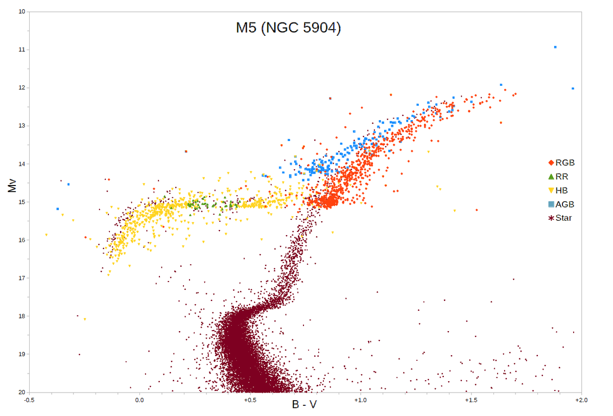
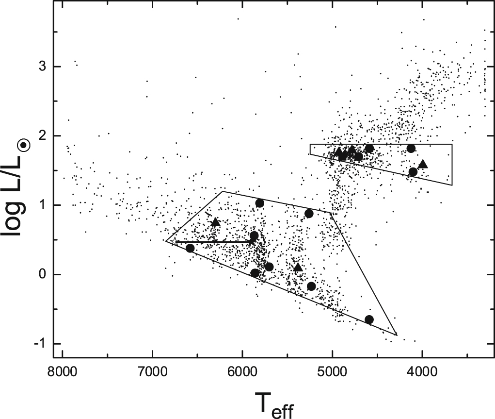
This H-R diagram for the globular cluster M5 shows where AGB stars lie: they are represented by blue markers here. The AGB is one of the final stages in a low- to intermediate-mass star’s lifetime. [Lithopsian]
But one particular stage of stellar evolution happens on timescales where we could see something happen, if we’re patient and watch for long enough: the end of the asymptotic giant branch (AGB). This is a stage at the end of a star’s life after it’s exhausted all of the hydrogen and helium in its core.
Low- to intermediate-mass stars aren’t able to ignite fusion of heavier elements in their cores, so at this stage, fusion proceeds only in a shell of hydrogen outside of the core. As the hydrogen shell burns, it piles up a thin layer of helium below it. But that quiet helium is deceptive: when enough of it piles up, it will ignite in a sudden flash called a thermal pulse, rapidly burning until the helium is depleted and the pile-up begins anew.
Rapidly, that is, on stellar evolution timescales — a typical thermal pulse lasts maybe a few hundred years, and these pulses occur only every 10,000 or 100,000 years. Still very difficult to observe on human timescales!

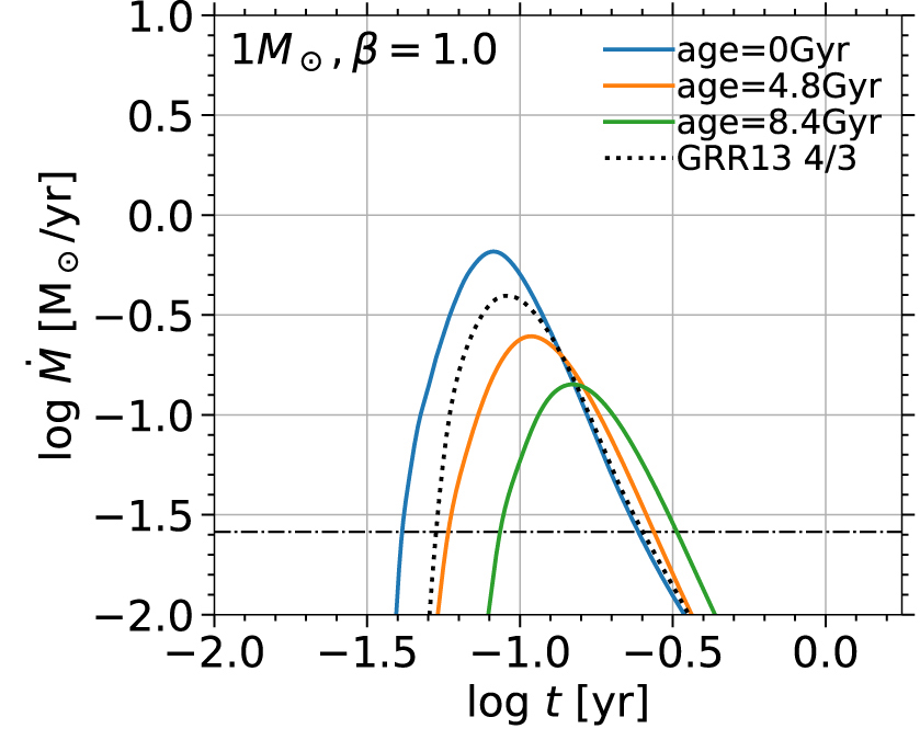
Example plot showing the radius change over time in a modeled star undergoing thermal pulses. Based on observational constraints of T UMi’s radius, the region of interest in this model for T UMi’s current evolutionary stage is marked in red. [Molnár, Joyce, & Kiss 2019]
Taking the Pulse of a Star
At the start of a pulse, the flash of igniting helium causes the inner regions of the star to expand. This, in turn, causes the outer parts of the star to cool and contract — so the star rapidly shrinks in radius and decreases in luminosity. If it’s a variable star — a star with periodic oscillations in brightness — the sudden drop in radius causes the period of its variability to plummet as the oscillating stellar envelope shrinks.
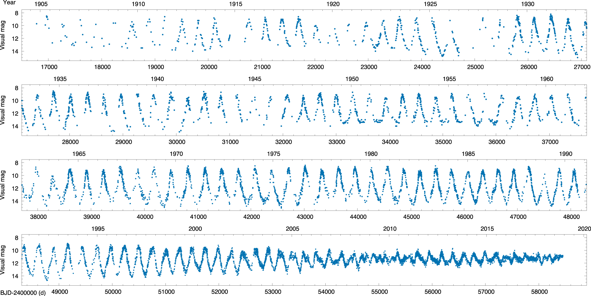
More than a century of data from variable star T UMi are shown in this AAVSO visual light curve. Changes in its period and amplitude are most evident in the bottom panel. Click to enlarge. [Molnár, Joyce, & Kiss 2019]
Using evolutionary and pulsation models, Molnár and collaborators confirmed that we’re indeed watching the onset of a thermal pulse in an AGB star. From their models, the authors predict that T UMi’s period will continue to drop for another several decades before the star begins to expand again — so be sure to check back in 50 years or so, to see if predictions pan out from this unique opportunity to watch a star evolve!
Citation
“Stellar Evolution in Real Time: Models Consistent with the Direct Observation of a Thermal Pulse in T Ursae Minoris,” László Molnár et al 2019 ApJ 879 62. doi:10.3847/1538-4357/ab22a5


