
A New Measurement of Turbulence
The same physical phenomenon that causes bumpy airplane rides also pervades our universe, jumbling stellar atmospheres, interstellar clouds, and even the magnetized sheath surrounding the Earth. Now, a new study brings us a little closer to understanding turbulence.
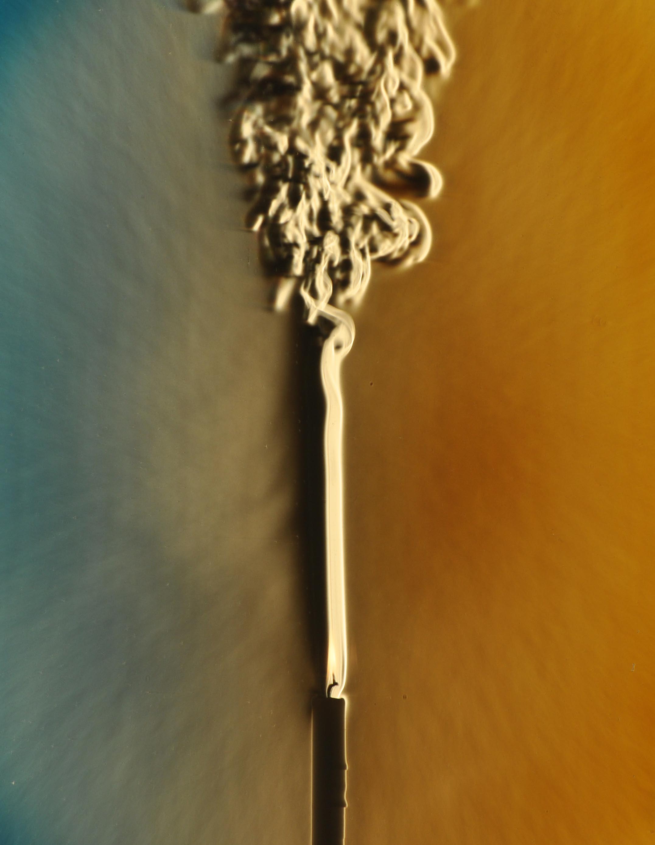
This image captures the transition between laminar and turbulent flow in the convection plume above a candle flame. [Gary Settles]
A Complex Phenomenon
Have you ever watched the entrancing wisps of smoke rising above a candle flame? What you’re looking at is turbulence — and despite this phenomenon’s prevalence throughout the universe, a complete description of turbulence remains one of the unsolved problems in physics.
The difficulty is that turbulent motion — characterized by rapid and chaotic fluctuations of fluid properties — is incredibly complex. Turbulence begins when energy is injected on large scales, causing field-level fluctuations. This energy then cascades down to smaller and smaller scales, creating chaotic motions all the way down to microscales. When the energy reaches small enough scales, it can dissipate, accelerating individual particles and converting into heat.
But scientists don’t fully understand the physical mechanisms at work in turbulence that inject the energy, transfer it to smaller scales, and eventually dissipate it. Worse yet, these processes take a different form when we’re no longer talking about fluids, but instead about astrophysical plasmas.
Plasmas, Plasmas Everywhere
Astrophysical plasmas are soups of ionized gas found everywhere from supernova remnants to the compressed solar wind surrounding the Earth in its magnetosheath — and in these plasmas, energy could be dissipated through a variety of mechanisms related to interactions between particles and waves.
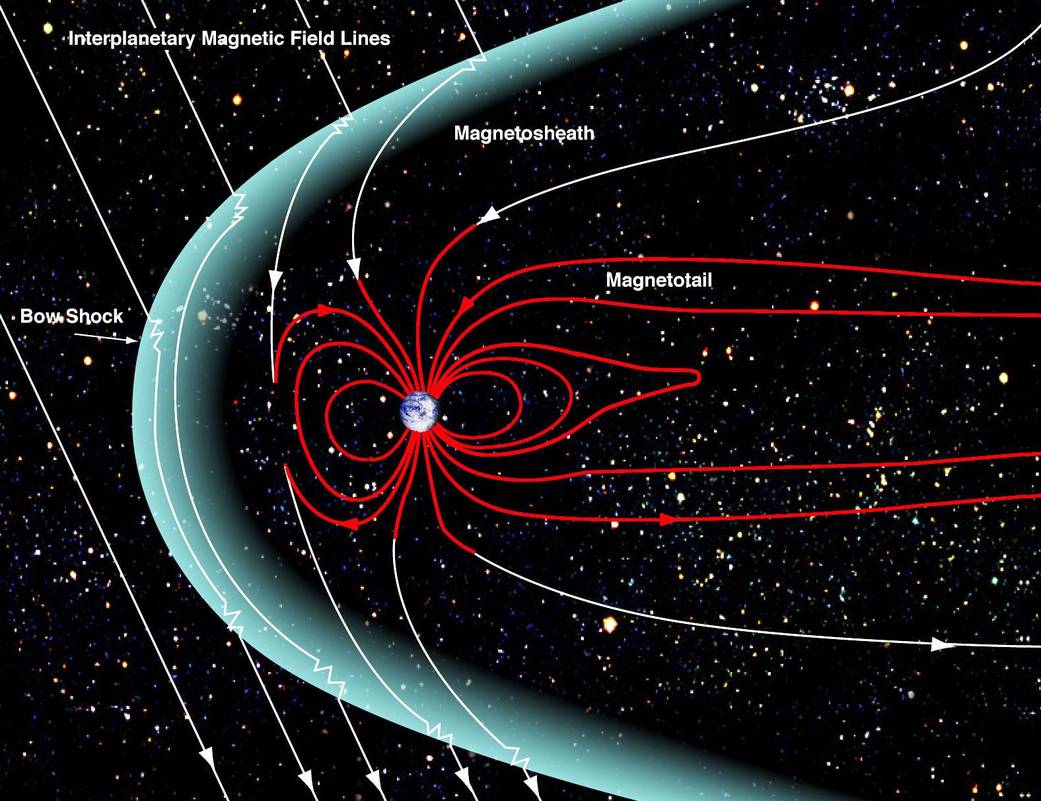
This diagram of the Earth’s magnetosphere shows the location of the magnetosheath, the region behind the bow shock where the compressed solar wind detours around the Earth. [NASA/Goddard/Aaron Kaase]
Measuring a Fluctuating Environment
The authors’ approach takes advantage of unprecedented, high-quality measurements made by the Magnetospheric Multiscale mission, a constellation of four spacecraft exploring the plasma environment around the Earth. As these spacecraft — separated by a distance of about 10 km — pass through magnetosheath plasma, they make measurements of the three-dimensional electric and magnetic fields, tracking the field fluctuations caused by turbulence.
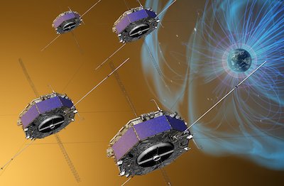
Artist depiction of the Magnetospheric Multiscale Mission spacecraft. [NASA/GSFC]
While we still have a lot to learn, He and collaborators’ work indicates that ion cyclotron waves — waves generated when ions oscillate in a magnetized plasma — play an important role in dissipating turbulent energy in the Earth’s magnetosheath.
More importantly, the authors’ approach for measuring the dissipation rates at different scales can be widely applied to different space plasma environments — so we can hope for more insight into turbulence in space in the future!
Citation
“Direct Measurement of the Dissipation Rate Spectrum around Ion Kinetic Scales in Space Plasma Turbulence,” Jiansen He et al 2019 ApJ 880 121. doi:10.3847/1538-4357/ab2a79


