Messier 87, or M87, is a massive elliptical galaxy that hosts one of the best-studied supermassive black holes in the universe. The black hole, commonly called M87*, was the subject of the first-ever photograph of a black hole, which was
released by the Event Horizon Telescope collaboration in 2019. Two years after that groundbreaking first photograph was revealed to the public, the collaboration
released a set of polarized images of the black hole, illuminating the magnetic field conditions close to the black hole and fueling years of research since.
Today’s Monthly Roundup explores three aspects of this supermassive black hole: how fast it spins, the properties of its relativistic jet, and the source of its powerful flares.
Taking M87’s Black Hole for a Spin
Spin is one of the fundamental parameters describing a black hole, along with mass and electric charge, and it’s a challenging quantity to measure. In a recent research article, Michael Drew (University of Central Lancashire) and collaborators used data from the Event Horizon Telescope from 2017 and 2018 to measure the spin of M87*. Their goal was to measure the angular momentum of the innermost region of the disk of material swirling around the black hole. For a 10-billion-year-old black hole like M87’s, the angular momentum of the inner reaches of the accretion disk is fundamentally linked to the spin of the black hole.
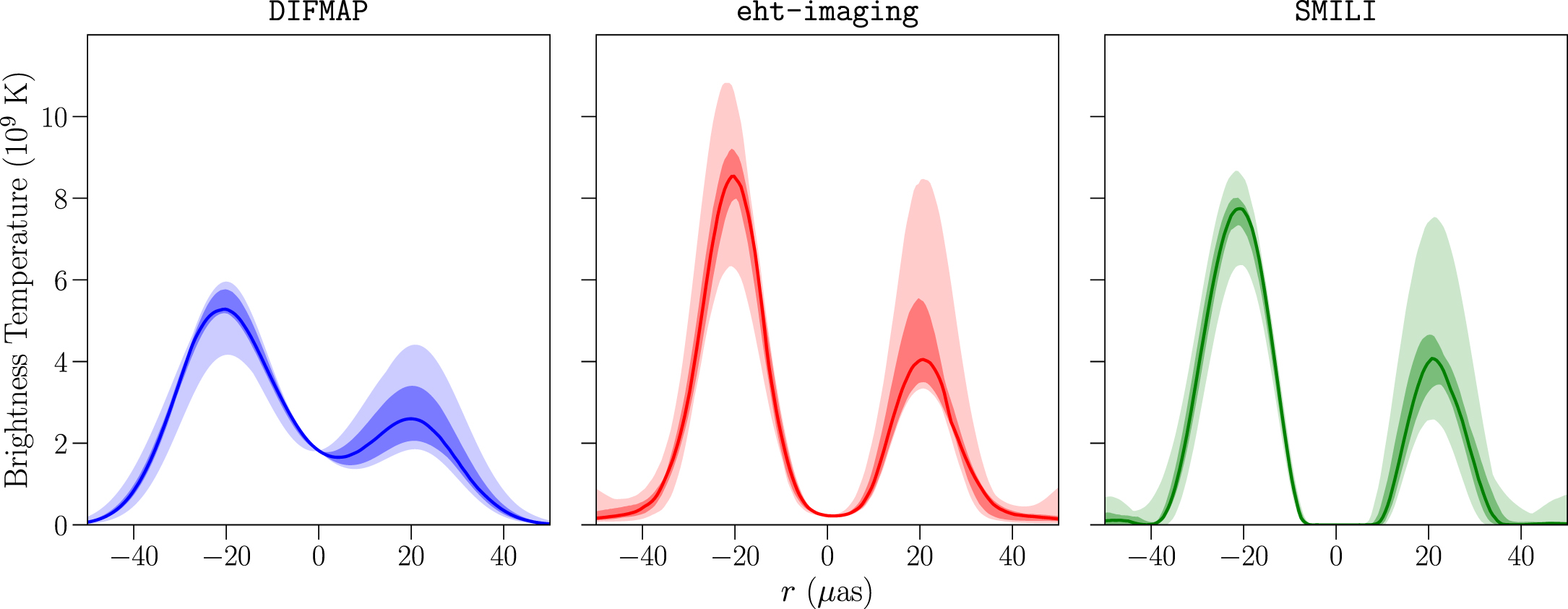
Radial brightness profiles of the Event Horizon Telescope images of M87*. The variation of the brightness of the ring is due in part to Doppler beaming. Click to enlarge. [Event Horizon Telescope Collaboration 2019]
The team’s measurement technique hinges on the existence of
relativistic Doppler beaming, which affects the apparent brightness of the fast-spinning material in the black hole’s accretion disk; material moving toward us as the disk rotates appears brighter, while material moving away appears fainter. By comparing the brightness of the brightest and faintest parts of the ring, Drew and coauthors estimated the velocity of the inner edge of the accretion disk. Combining this estimate with a measure of the disk’s inner radius from the Event Horizon Telescope yielded a measurement of the disk’s angular momentum and, by extension, the black hole’s spin.
This method returned a spin parameter of 0.8, which is within the broad range of previous estimates for M87*’s spin (0.1–0.98). Given certain assumptions made in this work, the team expects that this spin measurement is a lower limit on the black hole’s spin.
In addition to measuring the spin, the team also found a range of plausible accretion rates, from 4×10
-5 to 4×10
-1 solar mass per year (about 0.04–400 times the mass of Jupiter). These values are far below the theoretical maximum accretion rate for M87*, suggesting that while M87* is far more active than the black hole at the Milky Way’s center, it’s still fairly calm as far as black holes go. Finally, the team estimated the black hole’s accretion energy per unit time to be 6×10
33–6×10
37 Joules per second. These estimates largely overlap with existing estimates for the energy of M87*’s relativistic jet, supporting models in which the jet is powered by accretion.
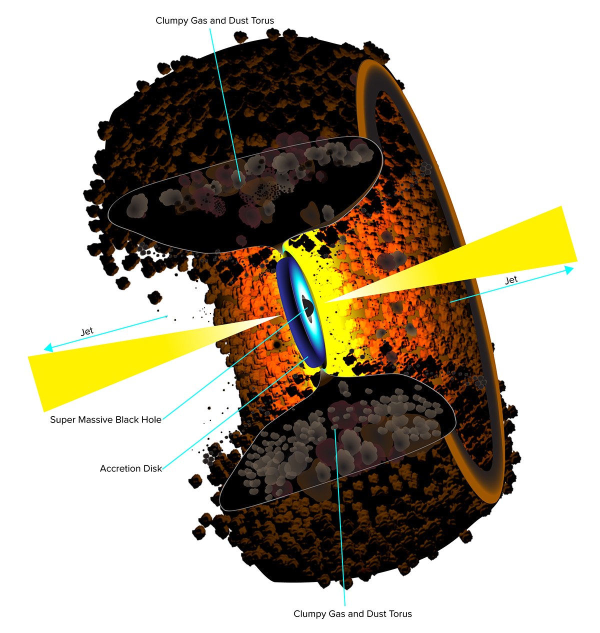
A New Model for Bright-Edged Jets
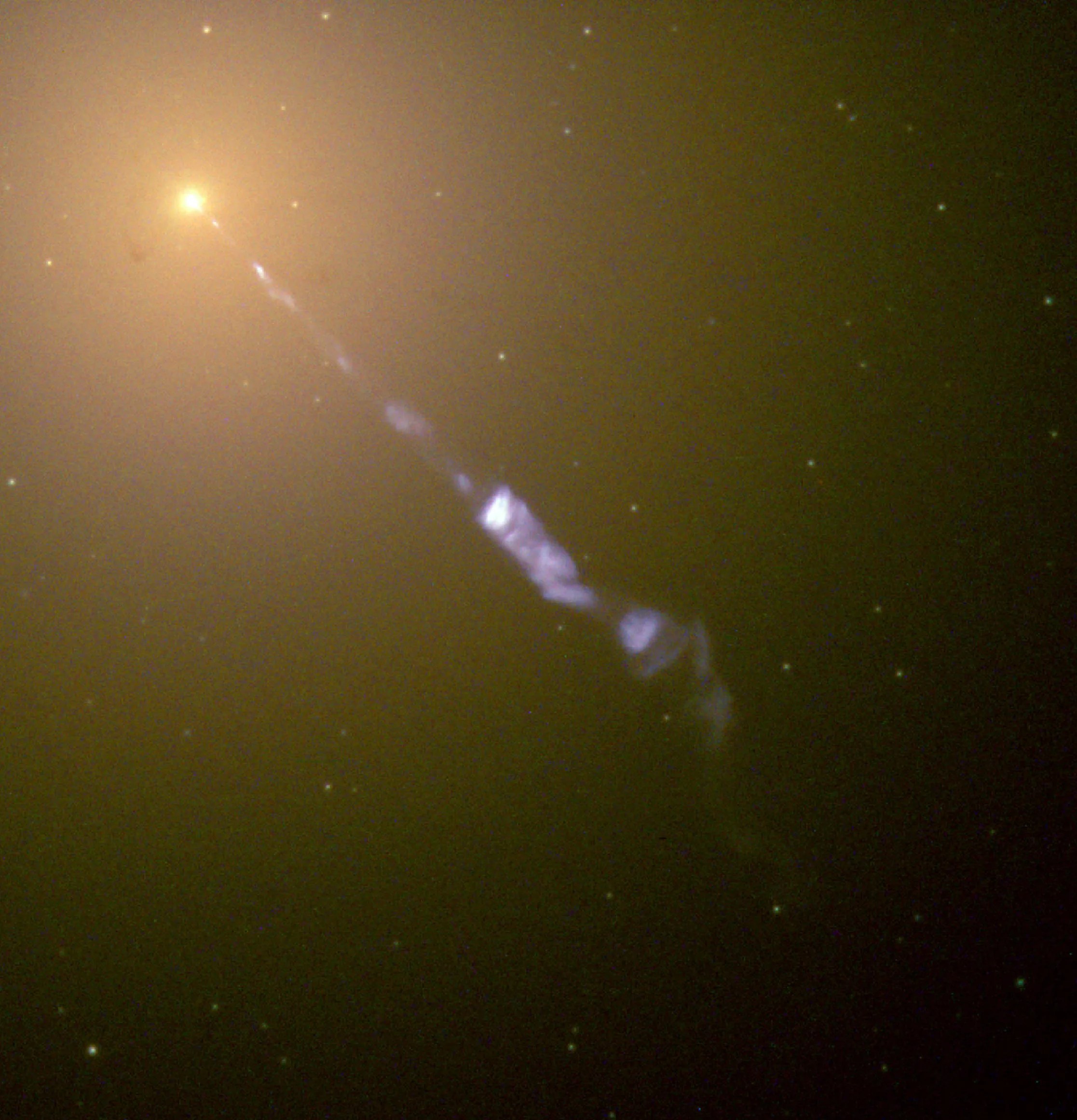
One of the most dramatic features of Messier 87 is its prominent jet. Researchers have noted that M87*’s jet exhibits limb brightening, meaning that the jet appears brighter along its edges than in its center. This characteristic is present throughout M87*’s jet, from close to the point at which it’s launched to far down its length, and is also seen in other black hole jets.
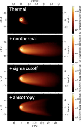
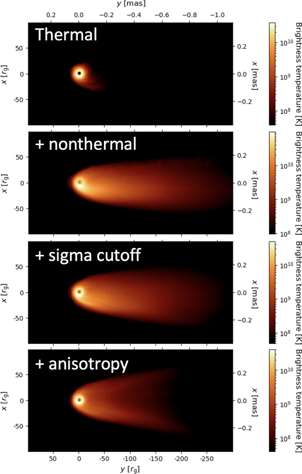
Demonstration of limb brightening in models that include an anisotropic electron distribution. [Tsunetoe et al. 2025]
So far, simulations have succeeded in producing a limb-brightened jet under carefully tailored conditions, but they have not yet managed to produce this feature across a range of scales and black hole spins. A team led by
Yuh Tsunetoe (Black Hole Initiative at Harvard University; University of Tsukuba) aimed to change that with their recent modeling study. The key feature of the team’s model is that the electrons that produce the jet’s prominent radio emission have much higher velocities parallel to the magnetic field lines that thread through the jet than perpendicular to the magnetic field (i.e., the electron distribution is anisotropic). Previous simulations using particle-in-cell methods, in which the behavior of individual particles is tracked, show that this anisotropic electron distribution is expected to arise in a relativistic, turbulent, magnetically dominated plasma.
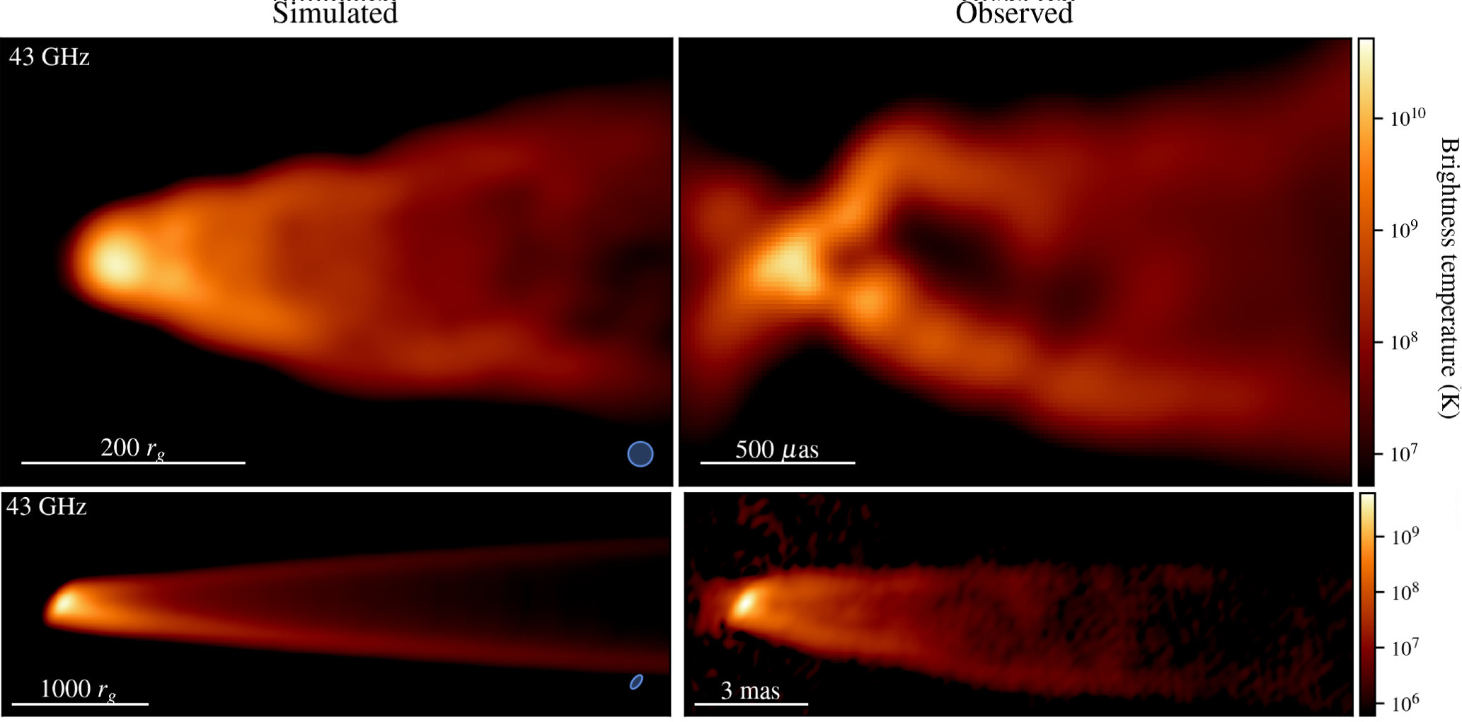
Tsunetoe’s team used both general relativistic magnetohydrodynamics (GRMHD) and general relativistic force-free electrodynamics (GRFFE) in their modeling. These two modeling techniques have different strengths and weaknesses: GRMHD allows time variations to be studied, but is only effective close to the black hole, while GRFFE applies at a large distance from the black hole, but can only give a time-averaged result. By combining these two methods, the authors were able to generate synthetic radio-frequency images of M87*’s jet and compare them to observations.
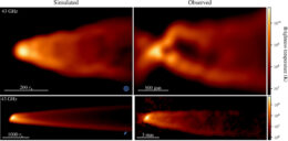
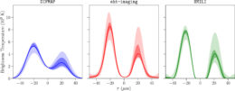
Simulated (left column) and observed (right column) jets. The top left shows the result from the GRMHD simulation and the bottom left shows the result from the GRFFE simulation. Note the difference in scale between the two simulations. Click to enlarge. [Adapted from Tsunetoe et al. 2025]
The resulting images show a clear limb-brightened jet across a wide range of both radio frequencies and spatial scales, as well as a striking resemblance to observations of the jet. In addition to comparing against existing data, Tsunetoe and collaborators produced images that can be compared against images from future facilities, such as the next-generation Event Horizon Telescope or the Black Hole Explorer. While more work remains to be done in the study of M87*’s jet — the team noted that their model doesn’t yet produce a counter-jet component as bright as what’s seen in observations — this work represents a significant advance in our ability to model the jets from supermassive black holes.
Investigating a Potential Source of Flares
Like many accreting supermassive black holes, M87* exhibits flares of high-energy radiation. These flares are highly variable, sometimes lasting only a couple of days, which suggests that they arise very close to the black hole’s event horizon. Precisely how these flares are generated is still unknown, though magnetic reconnection, in which magnetic fields rearrange and release pent-up magnetic energy, is a strong candidate.
Recently, Siddhant Solanki (University of Maryland) and collaborators investigated the source of M87*’s flares by tracing the paths of photons through a general relativistic magnetohydrodynamics simulation of an accreting spinning supermassive black hole. The simulation captured the region close to the black hole where magnetic reconnection is thought to occur, potentially launching electron–positron pairs that kick background photons up to high energies, powering a flare.
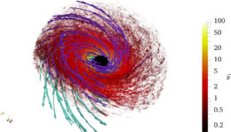
Illustration of the origin of the simulated flare emission. The majority of the emission arises from very close to the black hole. The purple and cyan curves indicate magnetic field lines. [Solanki et al. 2025]
By charting the course of individual photons as they depart from the current sheet — the surface that separates magnetic fields of opposite direction — and navigate the magnetized plasma surrounding the black hole, Solanki and coauthors show that much of the flux from the simulated flares arises within just 5 gravitational radii of the black hole. This supports the hypothesis that quickly varying flares are generated near the black hole’s event horizon.
The timescales of the simulated flares were also instructive. While the simulated flares tended to last about 130 days, each flare was composed of multiple smaller subflares, which lasted roughly as long as the rapid, ~2-day flares seen from M87*. If these flares are truly subflares arrayed within a longer-duration flare, Solanki and collaborators noted, they should have different time variability at long and short wavelengths. This suggests a need for long-term, multiwavelength monitoring of M87* to clarify the source of its flares.
Citation
“New Estimates of the Spin and Accretion Rate of the Black Hole M87*,” Michael Drew et al 2025 ApJL 984 L31. doi:10.3847/2041-8213/adc90e
“Limb-Brightened Jet in M87 from Anisotropic Nonthermal Electrons,” Yuh Tsunetoe et al 2025 ApJ 984 35. doi:10.3847/1538-4357/adc37a
“Modeling of Lightcurves from Reconnection-Powered Very High-Energy Flares from M87*,” Siddhant Solanki et al 2025 ApJ 985 147. doi:10.3847/1538-4357/adcba9