Editor’s Note: After a short hiatus, the Monthly Roundup is back! This series of articles, which began in 2023, examines multiple perspectives or findings on a single topic.
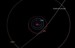
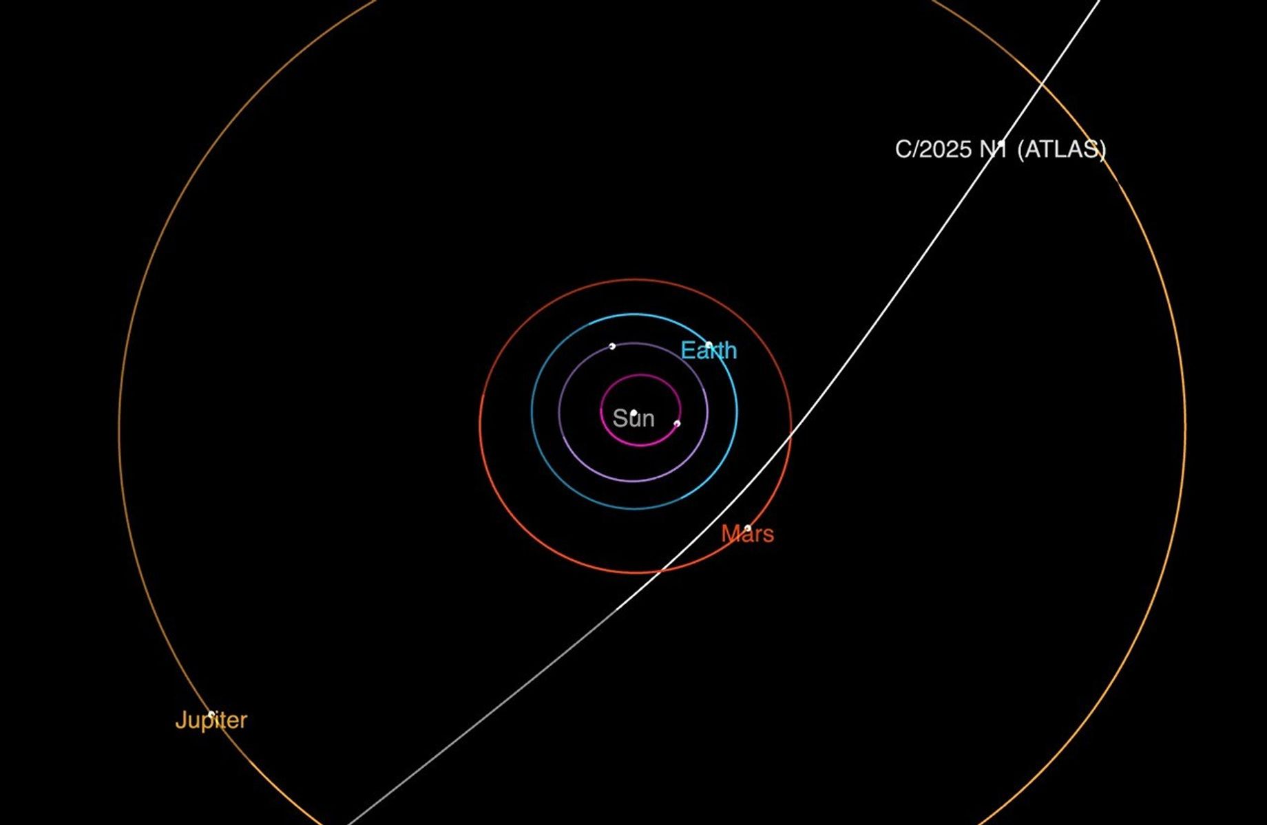
Interstellar object 3I/ATLAS’s trajectory through the solar system. Click to enlarge. [NASA/JPL-Caltech]
The discovery of interstellar object 3I/ATLAS on 1 July 2025 was one of last year’s top astronomy stories. First identified by the Asteroid Terrestrial-impact Last Alert System (ATLAS), 3I/ATLAS is just the third interstellar object that astronomers have seen speeding through our solar system; it was preceded by 1I/
ʻOumuamua in 2017 and 2I/Borisov in 2019.
Last summer, professional and amateur astronomers worldwide rolled out the red carpet in 3I/ATLAS’s honor, enlisting a pack of ground-based and spacefaring paparazzi to capture its every move. Observations in the first few months after 3I/ATLAS’s discovery revealed cometary features, including a fuzzy coma of gas and dust, a tail that trailed behind the object, and a plume of dust on the side facing the Sun.
With 3I/ATLAS having now made its closest approach to the Sun, venturing within 1.36 au of our star on 29 October 2025, the comet is wrapping up its tour of the solar system and heading back out to interstellar space — but the research continues. Today, we’re taking a look at five of the more than three dozen research articles published in the AAS journals that have examined 3I/ATLAS and its journey through our solar system. As always, this Monthly Roundup contains only a short summary of each article, so be sure to check out the full research articles linked at the bottom of this post!
Early Spectra of 3I/ATLAS
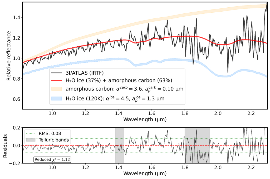
Bin Yang (Diego Portales University and the Planetary Science Institute) and collaborators obtained spectra of 3I/ATLAS less than two weeks after it was discovered, when it was 4.0–4.4 au from the Sun. Using the Gemini South telescope and the Infrared Telescope Facility (IRTF), Yang’s team sought to characterize its coma, the dusty envelope of gas that puffs out from the icy nucleus as the comet warms up.
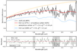
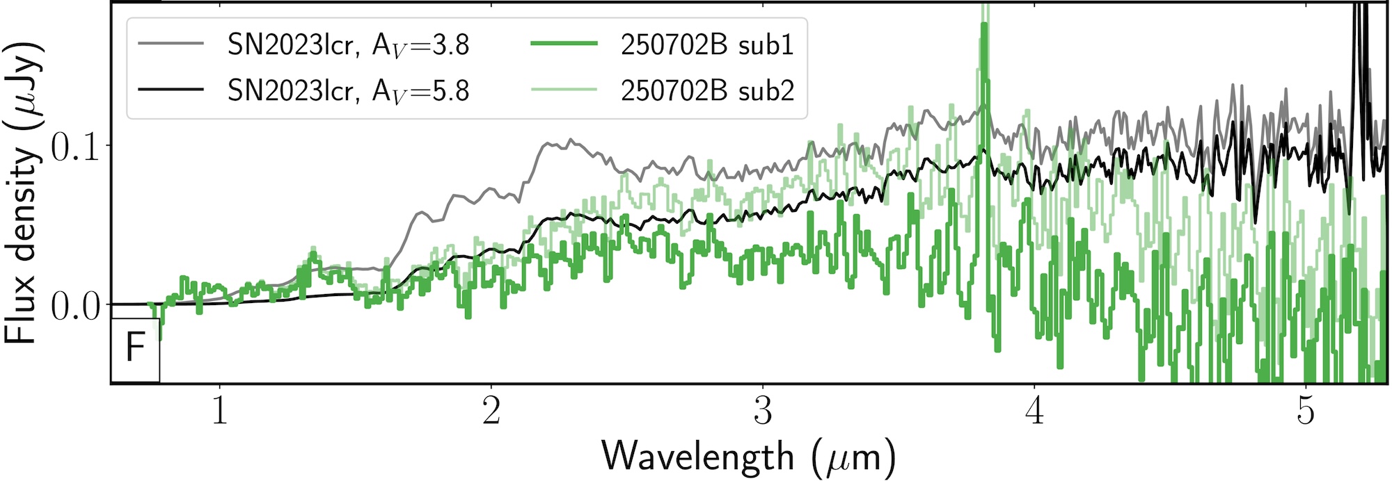
IRTF spectrum of 3I/ATLAS (black line) with the best-fitting model (red line). Click to enlarge. [Yang et al. 2025]
These observations showed that 3I/ATLAS has a relatively featureless, red-sloped spectrum from 0.5 to 0.8 microns, similar to certain asteroids and active comets in our solar system. In the near-infrared, 3I/ATLAS’s spectrum was flatter, with a broad absorption feature around 2.0 microns.
Yang and coauthors found that the near-infrared spectrum was well fit by a model including a blend of amorphous carbon and water ice (63% carbon and 37% water ice by volume) at a temperature of 120K. 3I/ATLAS’s spectrum bears certain similarities to well-studied solar system comets like C/2006 W3 and 6P/d’Arrest, which suggests that the particles in these objects’ comae are similar in size or composition. Ultimately, the discovery of abundant water ice in 3I/ATLAS’s coma, along with the carbon dioxide spotted in other studies, suggests that the comet formed in the cold, volatile-rich outer regions of its home system.
Unique Polarization Properties
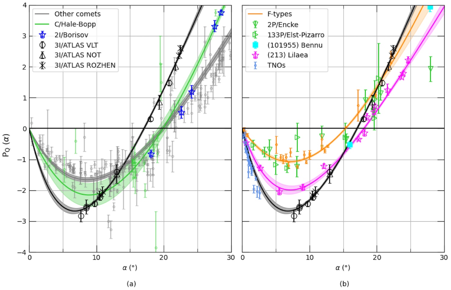
3I/ATLAS is the second interstellar object for which astronomers have obtained polarization information. The first, 2I/Borisov, showed a high degree of positive polarization, comparable to the exceptional solar system comet Hale–Bopp.
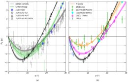
Comparison of 3I/ATLAS’s polarization (black) to measurements of 2I/Borisov (blue) as well as solar system comets and asteroids. Click to enlarge. [Gray et al. 2025]
Using the Very Large Telescope, the Nordic Optical Telescope, and the 2m Ritchey-Chrétien-Coude telescope to study 3I/ATLAS’s polarization between 17 July and 28 August 2025,
Zuri Gray (University of Helsinki) and coauthors showed that 3I/ATLAS is also exceptional — but in the opposite direction. In contrast to 2I/Borisov’s strong positive polarization, 3I/ATLAS is strongly
negatively polarized, with an unusually deep and narrow polarization profile. The narrowness of 3I/ATLAS’s polarization profile is similar to that of certain rare asteroids and cometary nuclei, but 3I/ATLAS is more strongly negatively polarized than these objects.
Gray’s team suggested that 3I/ATLAS’s extreme polarization behavior could be evidence for a mixture of large icy and dark particles in its coma. It’s also possible that it’s the first identified member of a new class of comets, distinct from both solar system comets and interstellar comet 2I/Borisov.
Is 3I/ATLAS Truly a Pristine Relic of the Star System It Came From?
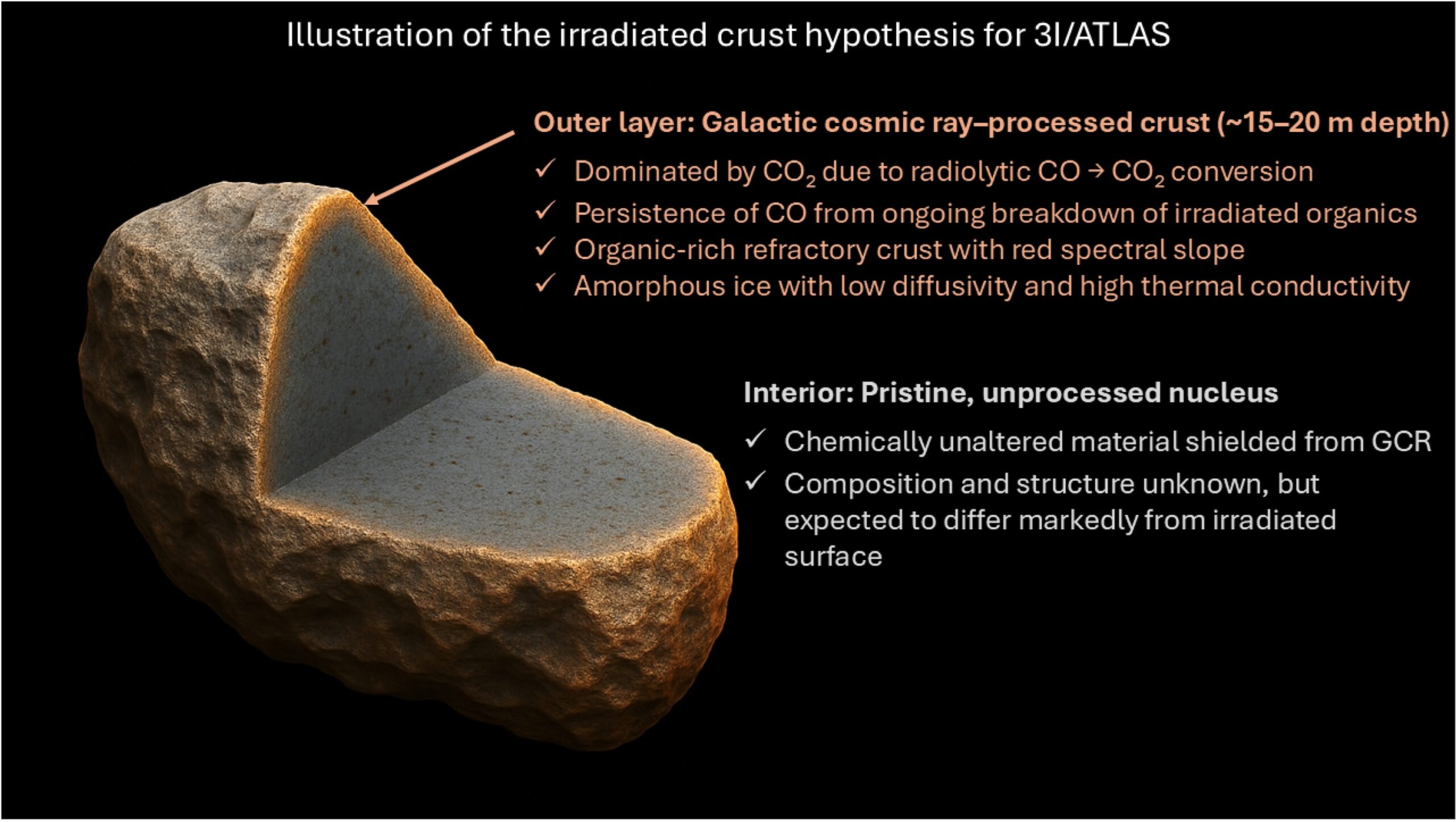
Interstellar objects like 3I/ATLAS have been hailed as pristine beacons that grant us a rare glimpse into the conditions of other star systems. But as new work by Romain Maggiolo (Royal Belgian Institute for Space Aeronomy) and collaborators shows, 3I/ATLAS was likely greatly altered by its journey through interstellar space.
Spectroscopic measurements from JWST suggest that 3I/ATLAS has extremely high abundance of carbon dioxide and carbon monoxide compared to water. A comet’s chemical abundance ratios can be either inherited from the material from which the comet formed, or they can be due to processing after its formation. The team finds that comet 3I/ATLAS’s extreme abundance ratios can be attributed to the comet being pummeled by galactic cosmic rays — high-energy charged particles — as it cruised through interstellar space.

Illustration of the nucleus of 3I/ATLAS, featuring a pristine core encased in a crust that has been irradiated by cosmic rays. Click to enlarge. [Maggiolo et al. 2026]
This means that 3I/ATLAS’s current composition doesn’t match its initial composition at the time of its formation, and the cosmic-ray-altered layer of the comet’s nucleus may be 15–20 meters thick. Could volatile outgassing and dust ejection scratch away enough of the comet’s outer layers to expose its pristine interior? This depends on the level of activity the comet experienced as it passed close to the Sun in October 2025. If the comet outgassed strongly, it could have shed tens of meters from its irradiated shell, exposing the pristine core material. Under low to moderate outgassing scenarios, however, the pristine inner material remains hidden beneath the processed shell. Now past the comet’s closest approach to the Sun, we’ll soon know more about whether the composition of the outgassed material has changed as the comet has moved through the solar system.
3I/ATLAS as a Template for Future Encounters: Planning a Potential Rendezvous
It’s only a matter of time before the next interstellar object pays our solar system a visit, and researchers are already thinking about how they’ll study the next visitor. One of the best ways to learn about an interstellar interloper would be to send a spacecraft to rendezvous with it and collect data from up close.
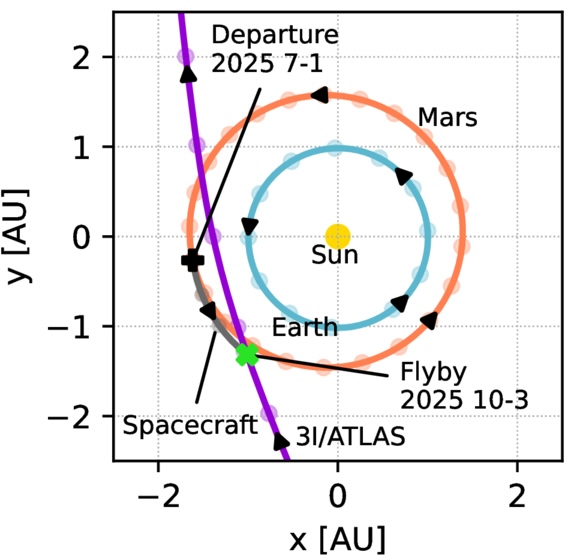
To plan for possible future rendezvous, Atsuhiro Yaginuma (Michigan State University) and collaborators considered what it would have taken for an existing spacecraft to meet up with 3I/ATLAS shortly after it was discovered. The team considered ready-to-launch spacecraft on Earth as well as operational spacecraft currently orbiting Mars.

Illustration of the trajectory for the minimum-energy rendezvous with 3I/ATLAS launched from Mars on the day the comet was discovered. [Adapted from Yaginuma et al. 2025]
Their calculations showed that meeting up with 3I/ATLAS from Mars would have required less energy than launching a new spacecraft from Earth, with Mars-originating flybys potentially possible with existing technologies. For Earth-originating flybys launched on or after the discovery date of 1 July, linking up with 3I/ATLAS is likely beyond current capabilities — but if the comet had been discovered earlier, a rendezvous launched from Earth
may have been possible.
This highlights the importance of detecting interstellar objects as early as possible, as well as the advantage of stationing well-fueled spacecraft at key locations around the solar system; these spacecraft could be deployed rapidly after an interstellar object is discovered, enabling the collection of valuable data. (This is similar to the premise of the European Space Agency’s Comet Interceptor mission, which will wait at one of the Sun–Earth Lagrange points for the arrival of a long-period comet; such a mission could be repurposed to track down an interstellar comet.)
So, About Those Aliens…
Like its predecessor 1I/ʻOumuamua, 3I/ATLAS prompted speculation that it’s not a natural object, though there’s no compelling evidence that it’s anything but a comet. If 3I/ATLAS were an interstellar probe, we might be able to unmask it as such by intercepting its radio communications. In a recent Research Note, Ben Jacobson-Bell (University of California, Berkeley) and coauthors described their search for narrow-band radio signals — the communication medium for all spacecraft in our solar system — from 3I/ATLAS.
The Breakthrough Listen project pointed the 100-meter Green Bank Telescope in 3I/ATLAS’s direction, just one day before the object made its closest approach to Earth at a distance of 1.8 au. The team identified nine possible “events” in their data, all of which were ruled to be radio-frequency interference. Based on this non-detection, Jacobson-Bell and collaborators ruled out the presence of isotropic, continuously outputting radio transmitters with power greater than 0.1 watt. (For comparison, a cellphone puts out approximately 1 watt, and spacecraft radios tend to put out a few dozen watts.) Other searches for radio transmissions from 3I/ATLAS have similarly detected no signals.
Citation
“Spectroscopic Characterization of Interstellar Object 3I/ATLAS: Water Ice in the Coma,” Bin Yang et al 2025 ApJL 992 L9. doi:10.3847/2041-8213/ae08a7
“Extreme Negative Polarization of New Interstellar Comet 3I/ATLAS,” Zuri Gray et al 2025 ApJL 992 L29. doi:10.3847/2041-8213/ae0c08
“Interstellar Comet 3I/ATLAS: Evidence for Galactic Cosmic-Ray Processing,” Romain Maggiolo et al 2026 ApJL 996 L34. doi:10.3847/2041-8213/ae2fff
“The Feasibility of a Spacecraft Flyby with the Third Interstellar Object 3I/ATLAS from Earth or Mars,” Atsuhiro Yaginuma et al 2025 ApJ 995 64. doi:10.3847/1538-4357/ae11b2
“Breakthrough Listen Observations of 3I/ATLAS with the Green Bank Telescope at 1–12 GHz,” Ben Jacobson-Bell et al 2025 Res. Notes AAS 9 351. doi:10.3847/2515-5172/ae3083


