Features RSS

map of the cosmic microwave background

The cosmic microwave background is leftover radiation from the Big Bang. It holds an enormous amount of information, and despite being from the beginning of the universe, it could tell us how the universe is going to evolve in the future.

Polarizing Measurements

One of the informative properties of cosmic microwave background (CMB) radiation is its polarization. In this case, polarization refers to how the component waves of the radiation are oriented relative to the direction the radiation is traveling in. Cosmological models are especially sensitive to the E-mode and B-mode polarizations of the CMB, where the E-mode is the component that is oriented parallel or perpendicular to the direction of travel while the B-mode is oriented at 45 degrees to the travel direction.

The E-mode of the CMB is especially interesting because it provides a measurement of the Hubble constant, a parameter that describes how quickly the universe is expanding. The Hubble constant can be measured in a variety of ways, and every technique ought to yield a similar value. However, this hasn’t turned out to be the case! The discrepancy between different measurements of the Hubble constant is an active area of research, and the E-mode-based value of the Hubble constant could help us understand the significance of this discrepancy.

We currently have three E-mode datasets to work with: one from the Planck satellite, one from the Atacama Cosmology Telescope ACTPol Receiver, and one from the South Pole Telescope SPTpol camera. We can derive individual measurements of the Hubble constant from each of these datasets, but what if we combined them? A study by Graeme Addison (Johns Hopkins University) does exactly that.

Modes and Models

Temperature fluctuations in the CMB and the overall distribution of normal matter (as opposed to dark matter) in the universe put the Hubble constant at about 67 kilometers per second per megaparsec. However, galaxy distances derived from variable stars and supernovae suggest the Hubble constant has a value of 73. These measurements are precise enough that there’s no overlap between their uncertainties.

The E-mode measurements of the Hubble constant made using each of the available datasets range from 70 to 73, though the uncertainty is larger than it is for the highest precision measurements. However, when all three datasets are combined, the value of the Hubble constant ends up being about 69, with a small enough uncertainty that the measurement is distinct from those made using galaxy distances. How could this happen?

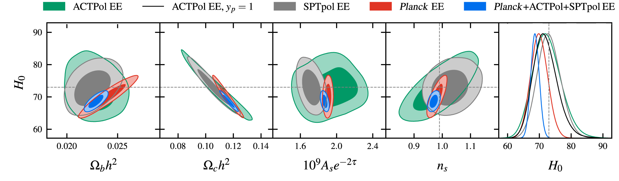
The Hubble constant plotted against various model parameters with different confidence intervals. The darker regions have a higher confidence than the lighter regions. The rightmost plot shows the range of values for the Hubble constant predicted for each dataset and the combination of all three datasets, with the distribution peaking at the likeliest value. The rightmost plot also contains two distributions for the ACTPol dataset, which have different assumptions. Click to enlarge. [Adapted from Addison 2021]

The answer probably lies in the constraints each dataset puts on different parameters of our dominant model of the universe. Each dataset suggests a slightly different range of values for each model parameter, which contributes to their predicted values of the Hubble constant. However, the “overlap” of these ranges points to a significantly lower Hubble constant than any of the individual datasets would suggest.

The bottom line is that the E-mode of the CMB seems to be in agreement with the CMB’s temperature fluctuations, which favors the current dominant model of the universe. The initial higher values of the Hubble constant could be caused by the inherent uncertainty in making observations of the CMB (it’s really hard!). At any rate, the discrepancy between different measurements of the Hubble constant continues to be a fascinating problem.

Citation

“High H0 Values from CMB E-mode Data: A Clue for Resolving the Hubble Tension?” Graeme E. Addison 2021 ApJL 912 L1. doi:10.3847/2041-8213/abf56e

Simulation showing two black holes in the process of merging. A star field makes up the background.

One way for black holes to form is in supernovae, or the deaths of massive stars. However, our current knowledge of stellar evolution and supernovae suggests that black holes with masses between 55 and 120 solar masses can’t be produced via supernovae. Gravitational-wave signals from black hole mergers offer us an observational test of this “gap” in black hole masses.

possible pair instability supernova

The supernova SN 2016iet, which might be one of the first observed pair-instability supernovae. The lines show the placement of the instrument used to take spectra of the supernova. [Adapted from Gomez et al. 2019]

Black Hole Boundaries

You need a massive star to go supernova to produce a black hole. Unfortunately, extremely massive stars explode so violently they leave nothing behind! This scenario can occur with pair-instability supernovae, which happens in stars with core masses between 40 and 135 solar masses. The “pair” in “pair-instability” refers to the electron–positron pairs that are produced by gamma rays interacting with nuclei in the star’s core. Energy is lost in this process, meaning that there’s less resistance to gravitational collapse.

As the star collapses further, two things can happen. If the star is sufficiently massive, its core ignites in an explosion that tears the star apart, leaving no remnant. If the star is less massive, the core ignition causes the star to pulse and shed mass till it leaves the pair-production stage and its core collapses normally into black hole. The most massive black hole that can be produced in this scenario is roughly 55 solar masses, forming the lower end of the black hole mass gap.

On the other side of the mass gap, it’s theoretically possible for certain massive stars to collapse normally without entering the pair-production state, thus evolving into black holes with masses greater than 120 solar masses. The unique thing about these massive stars is that they are low metallicity, containing practically no elements that are heavier than helium.

The likely masses of the black holes involved in the 46 mergers considered in this study. The x-axis is the expected mass of one black hole and the y-axis is the expected mass of the other. Each contour represents a merger. However, the bolded green and purple mergers represent the same merger, GW190521, and correspond to values from two different studies. The orange regions represent the predicted mass gap. [Adapted from Edelman et al. 2021]

So the bottom line is that we’re unlikely to observe any black holes with masses between 55 and 120 solar masses. But how can we test this prediction? Gravitational-wave signals are an option! Properties of merging black holes are coded into the gravitational waves produced by the merger, including the black hole masses. So, a recent study led by Bruce Edelman (University of Oregon) looked at our current catalog of black hole merger signals to see if the mass gap would emerge from the data.

Mind the Gap, If There Is a Gap

Edelman and collaborators used two established model distributions of black hole masses to approach the problem. They also altered the models so the gap was explicitly allowed and so higher black hole masses could be explored without artificially inflating the rate of mergers above the gap. Edelman and collaborators then fit their models to data from 46 binary black hole mergers observed by the Laser Interferometer Gravitational-Wave Observatory and the Virgo interferometer.

Interestingly, the existence of the gap is rather ambiguous! One factor is the inclusion of the merger associated with the signal GW190521, which was likely a high mass merger whose component black holes straddle the mass gap. If the gap doesn’t exist, it’s possible that the unexpected black holes are formed by the merging of smaller black holes. On the whole, this result points to many avenues of study when it comes to pair-instability supernovae and black hole formation!

Citation

“Poking Holes: Looking for Gaps in LIGO/Virgo’s Black Hole Population,” Bruce Edelman et al 2021 ApJL 913 L23. https://doi.org/10.3847/2041-8213/abfdb3

Composite photo shows an active galaxy with long, delicate filaments extending radially outward and forming loops and rings.

The dynamic environments around active galaxies often exhibit delicate filaments of cold gas. In a new study, scientists have explored how these fragile structures are able to form and survive within their hot, fast-moving surroundings.

Curious Structures

Image of NGC 1275 that contains outlines and insets identifying two particular filamentary structures

In this annotated image of NGC 1275 (click to enlarge), outlines and insets identify two filamentary structures: the blue loop (dotted outline and bottom left inset) and the horseshoe filament (dashed outline and top right inset). These two strikingly shaped filaments may both have been created during the same outburst. [Annotations: Yu Qiu]

The Perseus cluster, located more than 200 million light-years away, is a collection of thousands of galaxies embedded in a cloud of hot gas. At the cluster’s heart lies NGC 1275, an active galaxy that’s rapidly forming stars and contains an accreting supermassive black hole — two factors that result in outbursts of hot, fast outflows that are spewed into the intracluster medium.

In the midst of all this action, there’s a conundrum: we also see cold, outflowing gas that forms slender, elongated filamentary structures extending tens of thousands of light-years. Where does this cold gas come from, and how is it not heated or destroyed by the fast, hot outflows of the active galaxy?

Sweeping Up Old or Forming New?

Two explanations have been proposed for these cold outflows:

  1. The hot winds flowing from the active galaxy sweep up existing cold gas and carry it along, drawing it out into filaments.
    This idea has a challenge: long before the cold gas manages to reach the speeds we observe — more than 100 km/s! — it would likely be destroyed by shocks, preventing the formation of filaments.
  2. The cold gas forms within the hot outflows as these winds slow, cool, and fragment into filaments.
    This idea shows promise! In a new study, a team of scientists led by Yu Qiu (邱宇; Peking University, China) has explored this possibility further using a set of detailed simulations of an outbursting active galaxy.

Threads, Loops, and Horseshoes

Plots showing the shapes and speeds of cold gas in two simulations at three times. The shapes of the resulting filaments are very different in the two simulations.

The shape and speed of cold gas that forms within the outflows in two of the authors’ simulations (top and bottom) at three different times (left, middle, and right). The two simulations, which had different starting conditions, produce very different shapes of filaments: the top is long and threadlike, whereas the bottom is a perpendicular ring structure. [Qiu et al. 2021]

Qiu and collaborators’ 3D hydrodynamic simulations model a hot, radial outflow erupting from the center of a cluster similar to Perseus. From these simulations, the authors show how gravity and pressure from the surroundings cause the hot outflow to slow and cool. They confirm that this process eventually leads to fragmentation, forming filaments of cold gas that move at high speeds consistent with what we observe.

One especially interesting result of the authors’ work: the shapes of the resulting filaments depend strongly on the starting conditions of the outflow. This could explain some particularly striking shapes that we observe in Perseus — there are not only radial threads, but also a loop and a horseshoe at opposite sides of the central galaxy.

The authors show that a bipolar outburst with specific physical conditions can create two perpendicular rings of cold gas instead of long filaments — which could easily reproduce the loop and horseshoe we see in Perseus.

Qiu and collaborators demonstrate how we can use the morphology and locations of the filaments to probe the history of the active galaxy’s outbursts, inferring their energetics and properties. Further study of these delicate threads, loops, and horseshoes is sure to provide a wealth of new information about distant, active galaxies and clusters.

Citation

“Dynamics and Morphology of Cold Gas in Fast, Radiatively Cooling Outflows: Constraining AGN Energetics with Horseshoes,” Yu Qiu et al 2021 ApJL 917 L7. doi:10.3847/2041-8213/ac16d9

Illustration of a pulsar in the background exhibiting magnetic field lines looping between its poles. The pulse signal from this object extends into the foreground, where warped spacetime around a white dwarf causes the pulses to space out.

What does the inside of a neutron star — the incredibly dense remnant of an evolved star — look like? New observations of one of the most massive neutron stars provide some clues.

Mysterious Interior

Illustration of a bright white sphere with magnetic fields looping between its poles.

Neutron stars represent some of the most extreme environments in the universe. [Kevin Gill]

With the mass of multiple Suns packed into the rough size of a city, neutron stars represent one of the most dense, exotic environments in the universe. We can’t create an equivalent environment on Earth, so we rely on theoretical models — constrained by observations — to understand how matter behaves under these extreme circumstances.

Different theoretical models predict different interior structures for neutron stars, each described by an equation of state. In turn, each equation of state predicts a different maximum mass that a neutron star can reach before the overwhelming crush of gravity causes it to collapse into a black hole.

The heaviest neutron stars we spot in the universe, then, can help us to set upper limits and rule out some equations of state, narrowing down which models of neutron star interiors are most likely.

The catch? Measuring the precise masses of objects located thousands of light-years away is difficult! Luckily, the universe occasionally offers up clever tricks for doing so.

A Delay from Gravity

Some highly magnetized neutron stars emit beams of light that regularly pulse across our line of sight as they rotate. If these incredibly precise cosmic clocks — pulsars — have a binary companion, and if we view that binary edge-on, then we have a unique opportunity for some mass measurements.

Plot showing curves that describe the probability of the mass measurement for PSR J0740+6620.

The posterior distribution of PSR J0740+6620’s measured mass, using several different models. [Fonseca et al. 2021]

In such a system, the distortion of spacetime caused by the gravity of the companion object can affect the signal of the pulsar, such that the pulses arrive at Earth at slightly offset times. This effect, known as the Shapiro time delay, allows us to precisely measure the companion’s mass — which can then be used with the binary orbit to establish the pulsar’s mass.

In a recent study, a team of scientists led by Emmanuel Fonseca (McGill University, Canada; West Virginia University) have now used this approach with new observations of the pulsar PSR J0740+6620 to place the tightest constraints on its mass yet — and it’s a doozy.

Tipping the Scales

plot showing distribution of neutron star masses and histogram.

Mass distribution of neutron stars in known binary systems (click to enlarge). PSR J0740+6620 is currently the heaviest neutron star with a precisely measured mass. [Paulo Freire / Vivek Krishnan]

Fonseca and collaborators use observations from the 100-m Green Bank Telescope and the Canadian Hydrogen Intensity Mapping Experiment (CHIME) telescope to carefully model the Shapiro delay and measure the properties of PSR J0740+6620 and its companion, significantly improving upon previous measurements. The authors show that PSR J0740+6620 weighs in at 2.01–2.15 solar masses — confirming its status as the heaviest precisely measured neutron star currently known. They also confirm that the binary lies ~3,700 light-years away, and that the companion is an unusually cold white dwarf of just 0.25 solar mass.

Even more precise constraints — both on PSR J0740+6620 and other high-mass neutron stars — will be enabled by ongoing observations with currently technology, and by future studies using next-generation telescopes. Each improvement brings us a little closer to understanding the matter in these extreme objects.

Citation

“Refined Mass and Geometric Measurements of the High-mass PSR J0740+6620,” E. Fonseca et al 2021 ApJL 915 L12. doi:10.3847/2041-8213/ac03b8

Simulation of a black hole warping spacetime around it, with a background of the Milky Way.

Wandering supermassive black holes — those that don’t lie at their galaxies’ centers — may be tricky to find, but not all black holes that wander are lost! A new study demonstrates how we can hope to discover these missing nomads in the future.

Photograph of two spiral galaxies colliding.

When two galaxies collide, the resulting galaxy will contain multiple supermassive black holes. [NASA/Hubble Heritage Team (STScI)]

When Galaxies Collide

We know that the center of every massive galaxy hosts a supermassive black hole weighing millions to billions of solar masses. But galactic centers aren’t the only place that supermassive black holes can lurk! In fact, we expect that the majority of galaxies host many more of these monsters beyond just the central supermassive black holes. Why? Because galaxies merge.

Structure in our universe is largely built hierarchically: over time, galaxies have frequently collided with each other, growing progressively larger with each merger. But with each of these mergers, at least two supermassive black holes — one from each of the merging galaxies — are introduced into the resulting turmoil.

While gas and stars reorder themselves neatly into a new galaxy, eventually erasing all evidence of the merger, the black holes aren’t as well-behaved. Indeed, simulations show that it can take billions of years for those supermassive black holes to make their way to the center of the newly formed galaxy and merge — if they even make it at all!

Three simulated images show the stars, gas, and X-ray emission of a simulated galaxy that contains dozens of circled wandering supermassive black holes

This extreme example shows a simulated galaxy whose halo contains dozens of black holes (circled) above a million solar masses, including five (orange circles) shining with a bolometric luminosity above 1042 erg/s. The galaxy’s stars (top) and gas (center) show no evidence of the past mergers that led to this accumulation of black holes. The simulated X-ray image of the galaxy (bottom) reveals the five brightest black holes. [Adapted from Ricarte et al. 2021]

As more galaxy collisions occur, more off-center “wandering” supermassive black holes are produced — and by present day, galaxies can potentially host dozens of black holes above a million solar masses. So how do we find this vast population of wanderers? A new study led by Angelo Ricarte (Center for Astrophysics | Harvard & Smithsonian; Black Hole Initiative) explores the possibilities.

Revealing a Hidden Population

Ricarte and collaborators use a suite of cosmological simulations called ROMULUS to produce a realistic expectation of the black holes lurking in our universe. These simulations carefully track the positions and dynamics of supermassive black holes as galaxies merge and evolve over time, allowing us to explore the population of wandering supermassive black holes predicted to arise in galaxies at different times in the universe.

From this simulated population, the authors then predict the ways in which these wanderers may betray their locations:

  1. Hyperluminous X-ray sources
    Some nearby, accreting, wandering black holes should be detectable as exceedingly bright X-ray sources.
  2. Dual active galactic nuclei
    The simulations predict that galaxies will often host more than one dramatically accreting supermassive black hole — particularly at higher redshifts.
  3. X-ray halo
    If the black holes are too distant or dim to resolve individually, we can identify wanderers by stacking images of galaxies of similar mass. The “halo” of excess X-ray radiation can then be used to describe the wandering black hole population.
  4. Tidal disruption events
    Wandering supermassive black holes can tear apart stars that come too close! These disruptions should produce transient signals offset from galactic centers.

The ROMULUS simulations show that, for black holes smaller than 10 billion solar masses, wanderers greatly outnumber the central supermassive black holes in our universe. Ricarte and collaborators’ work demonstrates that we’ll need to consider this nomadic population carefully as we analyze our observations of the universe.

Citation

“Unveiling the Population of Wandering Black Holes via Electromagnetic Signatures,” Angelo Ricarte et al 2021 ApJL 916 L18. doi:10.3847/2041-8213/ac1170

Neutron Star Merger

The binary neutron star merger that produced GW170817 was also the source of a gamma-ray burst, which was unexpectedly faint. However, it turned out that this burst was not less energetic than average; rather, the jet that produced it had an unusual structure. So what caused the jet associated with GW170817 to look like it did?

A diagram showing the electromagnetic emissions arising from the binary neutron star merger that produced GW170817. The central jet that produced the GRB is offset from the line of sight by 30 degrees. [C. Bickel/Science]

Jet Setting Out of a Merger

The environment of a binary neutron star merger is a turbulent, energetic place. The merging objects can produce powerful winds and shed large amounts of mass, and the actual merger results in strong emission across the entire electromagnetic spectrum. The electromagnetic signal from the gravitational wave event GW170817 included the relatively short gamma-ray burst (GRB) 170817A, which turned out to be much fainter — and thus less energetic — than expected.

Some astronomers suggested that GRB 170817A belonged to a class of GRBs that were simply intrinsically less energetic, but others proposed that GRB 170817A was a typical short GRB — complete with polar jets launched after the collision — that was oriented off of our line of sight. Further study has borne out the latter prediction, but it has also shown that the jets associated with GRB 170817A have a somewhat unusual structure, especially toward their outer edges. What could cause this deviation from the norm?

To probe this question, a group of researchers led by Ariadna Murguia-Berthier (University of California, Santa Cruz/University of Copenhagen, Denmark) ran simulations of the winds and central jets involved in neutron star mergers to see how the structure of jets is influenced by their environments. 

Simulations of jets that were (top to bottom) choked, marginally successful, and successful. The parameter tw is the time the winds are active and tj is the time the central engine is active. [Adapted from Murguia-Berthier et al. 2021]

Breaking Free of Winds

There are several parameters to consider while modeling how a jet would move through a merger environment. Notably, it takes a finite amount of time for the merger remnant to collapse into (most probably) a black hole with an accretion disk. The collapse triggers the jet that would produce a short GRB. The surrounding winds are dependent on this collapse time, and their density could potentially snuff out the jet, preventing it from producing a short GRB. Murguia-Berthier and collaborators focused on how the jet would be affected by these winds and disk outflows.

A jet needs time to gather enough strength to break through the surrounding winds, so the central engine that powers the jet needs to stay active till the jet is strong enough. This balance between jet strength and wind strength plays a large role in whether a jet is successful in punching out of the merger environment and forming a short GRB. Additionally, while the jet is gathering strength and making headway into the winds, extra energy is deposited into a “cocoon” around the jet. This energy cocoon evolves based on its environment and can also impact the structure of the jet.

Merging with Observations

Murguia-Berthier and collaborators explored mergers with a variety of different parameters, but the parameters associated with GW170817 were of particular interest. The kilonova that accompanied the merger and the delay between the gravitational-wave signal and the GRB helped narrow down viable scenarios for the formation of this observed explosion. With their simulations, Murguia-Berthier and collaborators found that the time it took for the merger remnant to collapse into a black hole was between 1 and 1.7 seconds. Excitingly, this range agrees with many values from previous studies that used completely different approaches to estimate the collapse time!

Murguia-Berthier and collaborators cautioned readers that the simulations could not cover every physical scenario. However, this work is a demonstration of how simulations can be used with observational constraints to better explain the outcome of neutron star mergers.

Citation

“The Fate of the Merger Remnant in GW170817 and Its Imprint on the Jet Structure,” Ariadna Murguia-Berthier et al 2021 ApJ 908 152. doi:10.3847/1538-4357/abd08e

Map of the sky shows a bright band of gamma-ray emission across the center.

The disk of the Milky Way glows with continuous emission of high-energy gamma-ray photons. Where does this diffuse emission come from? A new study suggests that we may be missing the complete picture.

Smashing Cosmic Rays

Roughly 80% of the gamma-ray photons detected by the Fermi LAT gamma-ray detector come from diffuse emission — emission produced in the plane of our galaxy that isn’t associated with specific sources. Scientists have identified speeding cosmic rays as the primary culprit: high-energy protons and atomic nuclei whiz through space at nearly the speed of light, slamming into the interstellar medium and producing byproducts of gamma rays, neutrinos, and more.

Photograph of a detector array spread over a large surface of a plateau surrounded by mountains.

Observations from this cosmic-ray observatory in Tibet reveal the diffuse gamma-ray emission in our galaxy’s disk. [Institute of High Energy Physics of the Chinese Academy of Sciences]

But does this picture tell the whole story? In a recent study, Nanjing University scientists Ruo-Yu Liu and Xiang-Yu Wang point out a possible concern with this model: if cosmic-ray collisions produce the galaxy’s diffuse gamma-ray emission … where are all the neutrinos?

A Conflict from Missing Neutrinos

By modeling the interaction of galactic cosmic rays with the interstellar medium in the Milky Way, Liu and Wang illustrate the problem: in order to reproduce the spectrum of diffuse gamma-ray emission recently observed by detectors on the Tibetan Plateau, the cosmic-ray collisions would also produce a large number of neutrinos — so many, in fact, that they should be observable by detectors on Earth, like the IceCube neutrino observatory. The problem? Based on IceCube’s most recently released results, these predicted neutrinos aren’t there!

Since the neutrino and diffuse gamma-ray observations conflict, Liu and Wang argue, then the model must be missing something. The source of the seemingly diffuse gamma-ray emission from the galactic disk cannot only be cosmic-ray collisions with the interstellar medium. Instead, there must be a contribution from some additional source that produces high-energy gamma rays without also creating lots of neutrinos.

What is that source? The authors have found a potential culprit.

Another Player

Image of a complicated star-forming nebula with bright regions of gamma-ray emission

A grayscale infrared map of the Cygnus cocoon is overlaid here with colored gamma-ray data showing the excesses of high-energy photons. [IFJ PAN / HAWC]

Of the highest-energy diffuse gamma-rays detected by the Tibet observatory, 40% come from a single region: the center of the Cygnus cocoon, a superbubble surrounding a site of massive star formation. Could this area be producing the extra gamma rays observed in the diffuse emission?

Liu and Wang describe several potential sources of gamma rays in the cocoon — like the massive star cluster Cygnus OB2, the supernova remnant γ Cygni, and a pulsar wind nebula — and demonstrate that, by adding contributions from these sources, they can successfully reproduce the diffuse gamma-ray emission we observe while not exceeding the upper limits on neutrino production set by the IceCube observations.

More exploration of this picture is still needed, but the authors’ work shows that we still plenty more to learn about the sources that produce high-energy particles in our galaxy!

Citation

“Origin of Galactic Sub-PeV Diffuse Gamma-Ray Emission: Constraints from High-energy Neutrino Observations,” Ruo-Yu Liu and Xiang-Yu Wang 2021 ApJL 914 L7. doi:10.3847/2041-8213/ac02c5

Illustration of a disk of gas spiraling onto a bright protostar.

What forces are at work in the hidden centers of clouds that are forming baby massive stars? New images reveal the roles played by gravity and whirling magnetic fields.

To Make a Massive Star

High-mass stars of up to 120 solar masses are a critical driver of galaxy evolution: they pump energy into their surroundings and enrich galaxies with heavy elements that can’t be produced elsewhere. Yet massive stars remain shrouded in mystery — in fact, we still don’t fully understand how these behemoths are born.

young stellar objects

This false-color infrared image, captured by NASA’s WISE telescope, reveals young, massive stars (pink objects near center) forming in the Rho Ophiuchi cloud complex. [NASA/JPL-Caltech/WISE Team]

What do we know? The birthplaces of massive stars are molecular clouds that, as they collapse under their own gravity, fragment into clumps. Hot cores form at the centers of these clumps as collapse continues. Accretion disks then form around these molecular cores, feeding material from the collapsing cloud onto the soon-to-be star and helping it to grow to a point where nuclear fusion can ignite.

On scales of ~2,000–20,000 au, observations suggest that magnetic fields play an important role in funneling material inward to grow the baby star. But observations become more challenging to make on smaller scales — so we still don’t know what’s happening in the innermost ~1,000 au, at the interface between the molecular core and its accretion disk. Do magnetic fields provide useful support on these small scales? Or does gravity dominate, ultimately crushing everything inward?

Peering Into the Dust

In a new study led by Patricio Sanhueza (National Astronomical Observatory of Japan; SOKENDAI, Japan), a team of scientists has now addressed these questions. Using the incredible resolving power of the Atacama Large Millimeter/submillimeter Array (ALMA), Sanhueza and collaborators have probed the gas and dust at scales of ~1,000 au around a hot molecular core embedded in the high-mass star-forming region IRAS 18089–1732.

Image showing dust distributed into spiral filaments with correspondingly spiraling magnetic field lines.

ALMA observations show the dust (color scale and contours) and the magnetic field vectors at the center of the hot molecular core IRAS 18089–1732. [Sanhueza et al. 2021]

The high-resolution ALMA observations reveal spiral-like features in both the dust and the gas distribution in this innermost region — forming a seeming whirlpool of material falling inward onto the baby star. Using polarization measurements of the dust, the authors model the magnetic field to confirm that the field lines have been dragged around with the gas, producing a configuration that includes a toroidal component wrapping equatorially around the protostar.

Gravity Is King

What does all this tell us about the physical processes happening in the inner 1,000 au around a newly forming baby star? By analyzing the energy balance of the system, Sanhueza and collaborators show that gravity overwhelms the other processes at work in this region — including turbulence, rotation, and the magnetic field, which all play roughly equal roles in trying to support IRAS 18089–1732 against collapse.

Though magnetic fields exert an important influence on larger scales, they take a back seat in this innermost region where gravity is king. Thus, in the hot, shrouded centers of collapsing molecular clouds, even magnetic whirlpools eventually succumb to the crush of gravity to help form baby stars.

Citation

“Gravity-driven Magnetic Field at ~1000 au Scales in High-mass Star Formation,” Patricio Sanhueza et al 2021 ApJL 915 L10. doi:10.3847/2041-8213/ac081c

Image of two bright blue stars side by side and one dimmer circled star below, against a background of more distant stars.

Don’t plan to knock on a door at Alpha Centauri asking to borrow a cup of sugar just yet — but with a new look at this star system using a powerful telescope, we now know a bit more about our neighbors.

Secrets Among Nearby Stars

Proxima Centauri b

This artist’s interpretation shows the planet Proxima Centauri b around its host star. You can see the binary α Cen AB in between the planet and star, as two faint white dots in the background. [ESO]

When it comes to exploring Sun-like stars that might host planets, the Alpha Centauri (α Cen) star system is an ideal target. At just over 4 light-years away, this triple system — the binary pair α Cen AB and an additional companion, Proxima Centauri — contains the closest stars to the Sun.

Recent news has hyped the discovery of two exoplanets around the red dwarf Proxima Centauri — but what other surprises might the larger stellar system harbor? Given that α Cen A and B are both very similar to the Sun, it would be particularly valuable if we could find Earth-like, potentially habitable worlds around these near neighbors.

Choosing a Method

But how to detect them? Searching for transits works only for very specific orbit orientations. Direct imaging might be an option, since α Cen is so close. But even these nearby stars are challenging: α Cen A’s habitable zone lies at about 1.2 au, or just 0.9” in angular separation, from our point of view. It’s hard to confidently detect a small, dim object at that separation!

Four images of a single source in the center of a frame.

Calibrated images of α Cen A and B taken with ALMA in October 2018 (left two panels) and in August 2019 (right two panels). [Adapted from Akeson et al. 2021]

Another method may prove useful in this case, however: astrometry. In a new study, a team of scientists led by Rachel Akeson (NASA Exoplanet Science Institute, Caltech-IPAC) has used the high resolving power of the Atacama Large Millimeter/submillimeter Array (ALMA) to make some of the most precise astrometric measurements of α Cen AB yet.

Hints of Influence

Astrometry relies on the idea that the slight gravitational tug of an orbiting planet causes a star to “wobble” in place. If this effect is large enough, we can detect it via meticulous imaging that very precisely tracks the location and motion of the star on the sky over time.

Taking advantage of the high-resolution observations provided by ALMA’s long baseline, Akeson and collaborators captured measurements of α Cen A and B during 2018 and 2019. Their results provide the first high-accuracy absolute measurements of the stars’ positions on the sky since 1991, as well as the highest-accuracy differential astrometry yet, comparing their relative separation and searching for the tiny influence of planets around the two stars. 

Four-panel plot showing the best-fit orbit for the binary stars, a closeup of the data on the model, and the residuals.

Top left: astrometric measurements (red: Hipparcos and ALMA data, blue: archival data) and best-fit orbit of α Cen B relative to α Cen A. Top right: enlargement of the 2019 ALMA measurements (the total orbit takes ~80 years). Bottom: residuals of the fit as a function of time. [Akeson et al. 2021]

The authors then combine these results with archival data to better constrain α Cen AB’s orbit and properties.

A Promising Future

Akeson and collaborators show that ALMA can produce remarkably precise astrometric measurements for the α Cen system, demonstrating the exciting potential of using ALMA for this technique. Though the observations don’t reveal signs of a planet yet, continued monitoring should allow us to ultimately be able to detect planets of a few tens of Earth masses in stable orbits between 1 and 3 au around α Cen A.

But these results go beyond our search for planets — they also refine our measurements of α Cen’s motions. This allows us to make more accurate estimates of the physical properties of α Cen A and B, filling in our understanding of our nearest neighbors.

Citation

“Precision Millimeter Astrometry of the α Centauri AB System,” Rachel Akeson et al 2021 AJ 162 14. doi:10.3847/1538-3881/abfaff

Gaia spacecraft

The Gaia satellite is making the highest precision measurements yet of stellar movement. Specifically, it is measuring the positions, velocities, and parallaxes of stars across the sky. This is incredibly useful information to have, but it doesn’t provide a complete picture of a star’s motion. For instance, how do stars move along our line of sight?

A map showing the predicted paths of 40,000 stars over the next 400,000 years. The predicted paths are based on Gaia’s early third data release. The plotted stars are within 100 parsecs of the solar system. [ESA/Gaia/DPAC]

Not On All Dimensions

Currently, Gaia returns “5D astrometry” for most of the stars it observes, which consists of two position coordinates, two velocities, and a parallax (apparent change in position as the Earth orbits the Sun). A lot of science has been done with these data already, such as probing the origins of the stellar streams surrounding the Milky Way.

However, a majority of the astrometry provided by Gaia is restricted to the plane of the sky, which means we’re missing how stars move along our line of sight — that is, whether they’re moving towards or away from us. This puts some fascinating science out of reach, like mapping out subtle stellar and dark matter structures in the Milky Way. Spectroscopic surveys can give us line-of-sight velocities, but they are time-consuming and limited in the volume of space they can cover. Additionally, not many spectroscopic surveys overlap with the region being observed by Gaia.

All’s not lost though! A recent study led by Adriana Dropulic (Princeton University) shows how machine learning could be used to predict line-of-sight velocities for stars with 5D astrometry from Gaia.

The true, predicted, and error-sampled distributions of different stellar velocity components. The error-sampled distributions trace the true distributions more closely than the predicted distributions. [Adapted from Dropulic et al. 2019]

Training a Neural Network

To develop their machine learning technique, Dropulic and collaborators started with a publicly available catalog of mock Gaia data, which included line-of-sight velocities. They also added stars similar to those in Gaia Enceladus, a prominent stellar structure that emerges when velocities are plotted. The mock catalog ended up covering the space within roughly five kiloparsecs (or 16,000 light-years) of the Sun and contained roughly 75 million stars. The catalog was then separated into training, validation, and test sets, the former resembling the real Gaia sample that has line-of-sight velocities, or “6D” information. 

Dropulic and collaborators then trained a neural network to predict the line-of-sight velocity of a given star and the associated uncertainty with that velocity. An important caveat of this method is that it does not aim to make a near-perfect guess at the line-of-sight velocity for a single star. Rather, the goal is to get a reasonable estimate of the velocity distribution of a whole group of stars.

Moving On from Mock Data

An advantage of having the network output an uncertainty was that Dropulic and collaborators were able to construct “error-sampled” velocity distributions, which are produced by averaging multiple velocity and uncertainty predictions for a single star and repeating for the entire distribution. These error-sampled velocity distributions ended up being closer to the true distributions than the predicted distributions.

The next step in this work is to train the neural network on a real catalog of Gaia data and also explore more distant regions of the Milky Way. The upcoming third Gaia data release will contain roughly 30 million stars with full 6D astrometry, so it won’t be long till this machine learning method can be put into practice!

Citation

“Machine Learning the Sixth Dimension: Stellar Radial Velocities from 5D Phase-space Correlations,”  Adriana Dropulic et al 2021 ApJL 915 L14. doi:10.3847/2041-8213/ac09ef

1 51 52 53 54 55 119