Features RSS

intricate tendrils and clumps of gas and dust stretch across a star-forming region dotted with young stars

Astronomers have long attempted to understand why star-forming regions generate just a few high-mass stars while churning out many low-mass stars. Today’s article investigates a giant molecular cloud complex to understand the connection between dense, dusty cores and the stars that they form.

Scales Large and Small

map of hydrogen column density with thousands of cores marked

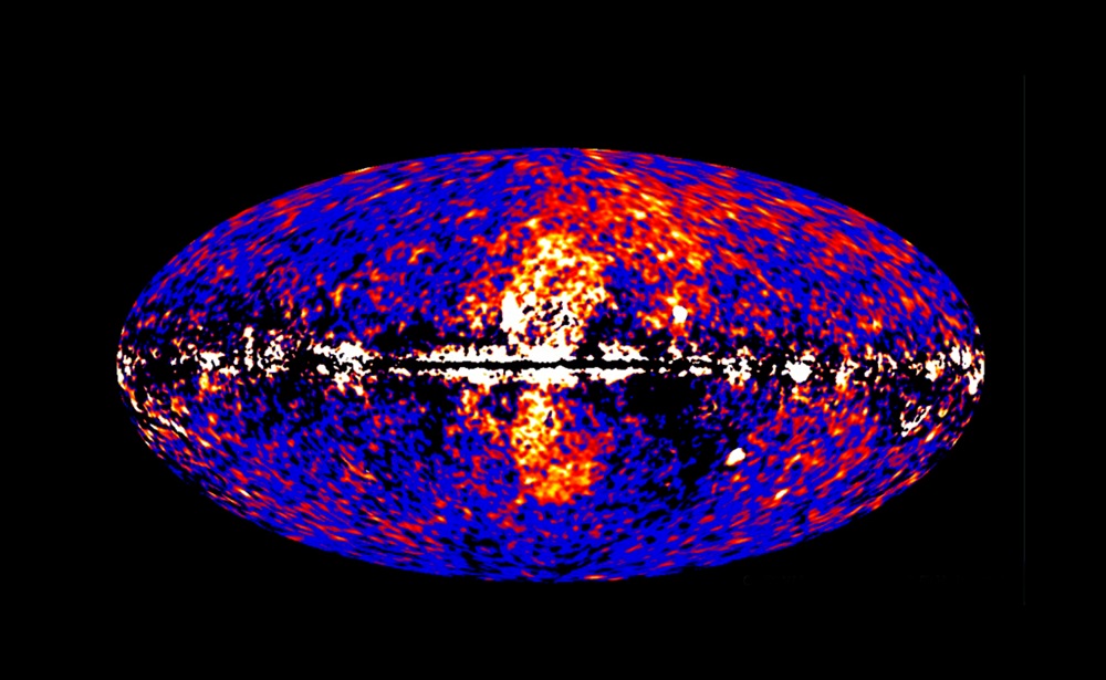
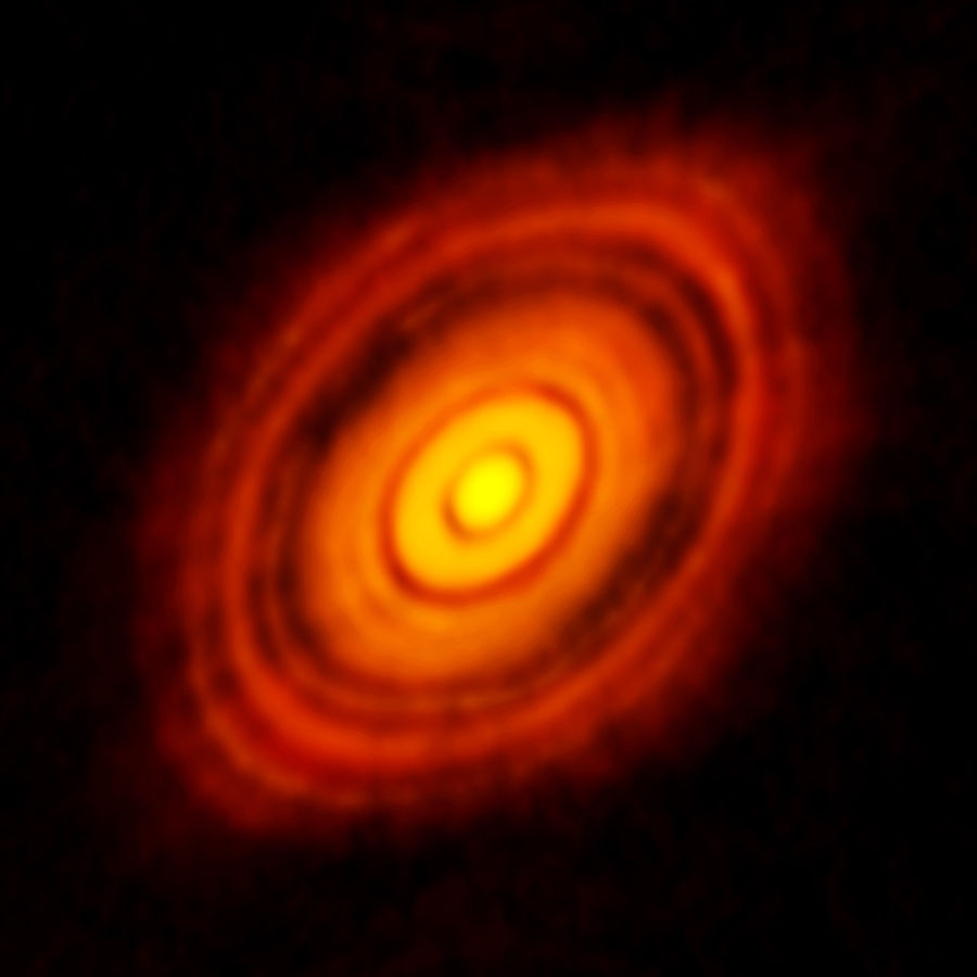
Thousands of cores (yellow ellipses) are visible in this hydrogen column density map of Cygnus X derived from Herschel Space Observatory data. Cores selected for later follow-up are indicated in red. [Cao et al. 2021]

When a giant molecular cloud begins to collapse, it forms dense cores. These cores fragment into even more condensed clumps that eventually become stars. But does the number of small and large cores directly predict the number of small and large stars?

Astronomers use the core mass function and the initial mass function to describe the number of cores and stars, respectively, that form in a molecular cloud as a function of mass. Thus far, observations indicate that the core mass function and the initial mass function both show the same strong preference for forming small objects over large ones, leading astronomers to suggest that the functions are closely related. To test this picture and explore the roots of this relationship, a team led by Yue Cao (Nanjing University, China) has now dramatically expanded our sample of star-forming cores by analyzing observations of the enormous Cygnus X giant molecular cloud complex.

An Extensive Search

In order to determine the core mass function precisely, Cao and collaborators needed a large sample of cores. Their search brought them to the Cygnus X star-forming region: a 650-light-year-wide molecular cloud containing three million solar masses of gas and dust and home to thousands of star-forming cores.

core mass function derived in this work versus two existing initial mass functions

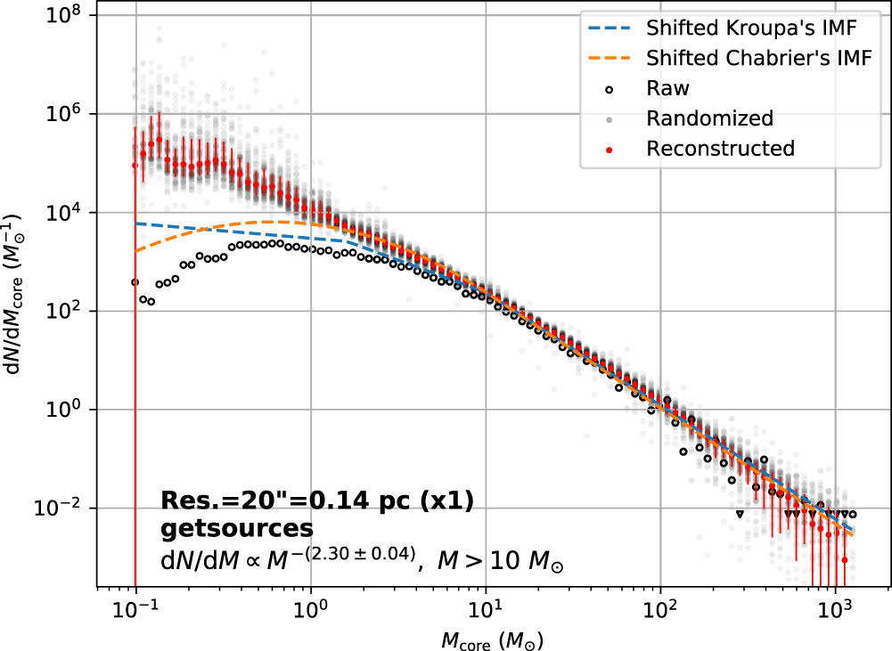
Corrected core mass function for Cygnus X (red symbols) compared against the uncorrected core mass function (black symbols) and two initial mass functions (IMFs; dotted lines). [Cao et al. 2021]

Cao and collaborators used a search algorithm to identify cores in far-infrared and submillimeter observations of the Cygnus X cloud complex. In total, they selected 8,431 cores with masses ranging from just a tenth of a solar mass to more than a thousand solar masses, making this the largest sample of star-forming cores in a single cloud complex analyzed to date.

After accounting for biases in their search algorithm, the authors found that while the core mass function generally follows the same shape as the initial mass function, there are discrepancies at both mass extremes; Cygnus X has more low-mass cores and fewer high-mass cores than expected if the core mass function is directly related to the initial mass function. This contradicts findings from smaller studies of star-forming regions, which found greater agreement between the shapes of the two mass functions.

From Cloud to Core to Condensation

greyscale images of four cores with contours of the hydrogen column density and ellipses marking the diameters of the cores

Selected observations of cores. Hydrogen density contours are in yellow, core diameters are in red, and condensations are marked with cyan crosses. [Adapted from Cao et al. 2021]

The authors pushed their investigation to even smaller scales by performing follow-up observations of 48 cores with the Submillimeter Array. Using these highly detailed observations, they searched for substructures in the cores called condensations, finding 180 in total. The authors find no correlation between the core masses and the condensation masses, indicating that there isn’t a simple relation between them.

Overall, these results indicate that the initial mass function doesn’t arise directly from the core mass function, perhaps due to the chaotic influence of turbulence in star-forming regions. As always, star formation is anything but simple!

Citation

“Core Mass Function of a Single Giant Molecular Cloud Complex with ∼10,000 Cores,” Yue Cao et al 2021 ApJL 918 L4. doi:10.3847/2041-8213/ac1947

hundreds of densely packed glowing stars with some faint nebulosity

A leading theory for how massive (and supermassive) black holes form is hierarchical merging — the idea that massive black holes are built from a series of collisions between lighter black holes. Densely packed environments like globular clusters and nuclear star clusters at the centers of galaxies are expected to be prime sites for black-hole mergers, but gravitational-wave “kicks” might get in the way.

Get a Kick Out of This

When black holes merge, they emit gravitational waves that carry away energy and momentum. The waves aren’t emitted equally in all directions, so the act of merging imparts a “kick” to the merger product. It’s far from a gentle nudge — typical kick velocities are estimated to be hundreds or thousands of kilometers per second. If a black hole gets a big enough kick, it can leave the dense cluster it formed in and emerge into rarefied space, where it’s far less likely to undergo further mergers. How typical is it for black holes to get ejected from their nascent star clusters, and what does it mean for the theory of hierarchical merging?

probability density functions for the kick velocities of four black-hole mergers

Probabilities of five merger products having a given kick velocity. [Adapted from Mahapatra et al. 2021]

Current gravitational-wave detectors aren’t sensitive enough to detect the ejection of a black hole directly, but we can infer the kick velocity from the gravitational waves we observe. A team led by Parthapratim Mahapatra (Chennai Mathematical Institute, India) applied mathematical models to data from 47 black-hole mergers detected by LIGO and Virgo to investigate the likelihood of black holes being kicked out of different types of star clusters. The authors estimated each event’s kick velocity, which depends on the ratio of the masses of the merging black holes, their spin rates, and other factors.

retention probability as a function of escape velocity with typical escape velocities for globular clusters (2-180 km/s) and nuclear star clusters (

Retention probability as a function of cluster escape velocity for several gravitational-wave events in the catalog. The grey lines correspond to five of the six merger events that showed signs of previous hierarchical mergers; the red dotted line is the sixth. [Mahapatra et al. 2021]

Globular vs Nuclear

Mahapatra and coauthors used their estimates to determine the probability of a merger product remaining in the cluster in which it formed as a function of the cluster’s escape velocity, finding a wide range of retention likelihoods. The authors pay special attention to the six events in the catalog that show signs of being the products of previous hierarchical mergers, like GW190521 — the most massive black-hole merger detected so far. They estimate that a merger like GW190521 would have a 50% chance of remaining bound to a star cluster that had an escape velocity of 700 km/s. Since this escape velocity is well within the expected range for nuclear star clusters, this means that if GW190521 were housed in such a dense environment, its massive product may well merge again in the future.

Ultimately, it’s clear that some star clusters are better at retaining post-merger black holes than others. Given their low escape velocities, globular clusters are unlikely to be the sites of repeated mergers; of the 40 cataloged mergers with the best data, the authors estimate that 17 would be retained by nuclear star clusters and only 2 would be retained by globular clusters. Without knowing more about the environments in which these mergers took place, it’s impossible to say whether an individual merger product will escape from its surroundings, but the authors’ findings have important implications for where hierarchical merging is likely to take place generally.

Citation

“Remnant Black Hole Kicks and Implications for Hierarchical Mergers,” Parthapratim Mahapatra et al 2021 ApJL 918 L31. doi:10.3847/2041-8213/ac20db

gas-giant formation

CI Tauri is thought to host a massive planet roughly five times closer than Mercury is to the Sun, but observations reveal ample radiation arising from gas and dust close to the star — gas and dust that we would expect to be missing if a planet were present. Can astronomers explain these conflicting observations?

CI Tau continuum observations

Synthesized image of CI Tau continuum observations, revealing three annular gaps between 10 and 100 AU. The inset shows a 0.35”-wide zoom on the innermost gap, imaged with a finer resolution. [Clarke et al. 2018]

Protoplanetary Problems

At just 2 million years old, CI Tauri already has a 12-Jupiter-mass planet, CI Tau b, orbiting at just 0.08 au, and three additional giant planets potentially lurk in CI Tauri’s disk at tens of au. Curiously, though, the system’s spectral energy distribution — the amount of energy emitted as a function of wavelength — lacks the tell-tale sign of a close-in massive planet: a dip in the amount of near-infrared emission, which is produced by warm gas and dust.

Much of the 1–10-μm radiation from a protoplanetary disk arises from the material closest to the star, so a decrease in emission at these wavelengths is usually taken as a sign that a close-in planet is busily scooping up gas and dust to carve out a gap in the disk material. However, observations of CI Tauri suggest that a planet could be present without changing the near-infrared emission. To test this, Dhruv Muley and Ruobing Dong (University of Victoria, Canada) used hydrodynamic and radiative transfer modeling to understand the conditions under which a close-in planet will affect the system’s spectral energy distribution.

hydrodynamic simulation of planets accreting material

An example simulation of a planet (smaller white circle) with an orbital eccentricity (ep) of 0.4. The color indicates the particle density and the dotted lines show the regions where the planet is able to accrete material. [Adapted from Muley & Dong 2021]

Disks, Dust, and Distributions

The authors first modeled a disk with no planets present, matching the model output to the observations of CI Tauri as closely as possible. Next, they introduced a CI Tau b-sized planet into the simulation and gave it time to carve a swath through the disk before comparing the outcomes for a range of orbital distances and eccentricities. Muley and Dong found that planets with more elliptical orbits create gaps that are wider, since they’re able to collect material within a larger range of radii, but the material that remains in the gap is denser than it would be in the case of a planet with a perfectly circular orbit.

The authors then used their hydrodynamic simulations to generate a spectral energy distribution for each set of conditions. They found that a planet at CI Tau b’s orbital distance of 0.08 au doesn’t remove enough material to induce the tell-tale dip in the near-infrared emission, regardless of its eccentricity, which is consistent with the observations.

simulated spectral energy distributions

Simulated spectral energy distributions showing the effects of the planet’s orbital distance (ap; varies between panels) and eccentricity (ep; varies with line color). [Muley & Dong 2021]

Impactful Conditions

However, a CI Tau b-size planet placed slightly farther from the star — say, 0.26 or 0.40 au — makes its presence known in the resultant spectral energy distribution. The more distant planets deplete the disk material enough to decrease the 1–10-μm emission and open gaps wide enough to reveal the hot inner wall of the gap, which increases the emission at 10–100 μm.

The authors’ simulations show that the presence of a close-in planet isn’t at odds with CI Tauri’s spectral energy distribution, and more generally, a lack of typical planetary indicators might not signal a lack of planets. Since spectral energy distributions are one of our most powerful tools for studying protoplanetary disks, it’s crucial to understand their intricacies in order to trust our interpretations.

Citation

“CI Tau: A Controlled Experiment in Disk–Planet Interaction,” Dhruv Muley and Ruobing Dong 2021 ApJL 921 L34. doi:10.3847/2041-8213/ac32df

A pulsar timing array

Deep within the universe, supermassive black holes are swirling around each other, giving off an immense amount of energy that travels at the speed of light through a fabric of ticking stellar clocks. Have we been looking long enough to catch their distant background whisper?  

In 2015, LIGO announced the first detection of ripples in the fabric of spacetime, and since then, scientists have detected ~90 gravitational-wave events (35 of which were announced this week!), consisting of black hole–black hole mergers, neutron star–neutron star mergers, and black hole–neutron star mergers. These different sources each produce their own frequency of gravitational waves depending on the mass of the object. For instance, binary neutron star mergers are very energetic and happen quickly, so they produce high-frequency waves, but mergers of supermassive black hole binaries happen much more slowly and generate much weaker, low-frequency waves. Much like how you can’t detect a gamma-ray burst with an infrared telescope, you can’t observe gravitational waves from binary supermassive black holes with something meant for binary neutron star mergers. This is where pulsar timing arrays come in.  

A Galaxy-Sized Gravitational Wave Detector

Different periods of gravitational waves and what instruments can detect them

Different frequencies of gravitational waves that can be detected by various instruments that can detect them (left to right: BICEP2, the Green Bank Telescope LISA, LIGO). [Shami Chatterjee/NANOGrav]

Pulsars are super dense, rapidly rotating neutron stars that emit radio radiation that crosses our sightline like a lighthouse as the star spins. Pulsars are incredibly periodic and rival atomic clocks in terms of precision, so we can predict exactly when a pulse will arrive. Pulsar timing arrays are collections of millisecond pulsars (which are especially stable and spin hundreds of times per second) around the sky that are monitored for changes in the time of arrival of their pulses. Because they’re scattered throughout the galaxy, a pulsar timing array is essentially a galaxy-sized gravitational wave detector. If a gravitational wave comes between us and a pulsar, it will show up in the pulse arrival times because the distance between the pulsars will have changed slightly as space is stretched and squeezed by the wave.  

When searching for gravitational waves, the goal is not only to detect them but also to characterize them. The passage of a gravitational wave changes the arrival times of pulsar signals in a distinctive way that can be described by something known as the Hellings–Downs curve. By obtaining many times of arrival from pulsars all around the sky, astronomers can look for signs of this curve and use it to characterize the source of the gravitational waves. 

Angle between pulsars vs. the correlation between their times of arrival

The Hellings–Downs Curve, which plots the separation between pulsars against the correlation between their arrival times. If a gravitational wave passes between through, it will show up in the times of arrival between different pairs of pulsars on the sky and follow this curve exactly. [Mike Zevin/Astrobites]

Hunting for the Hellings–Downs

But this is easier said than done! The gravitational waves that can be detected by timing arrays are incredibly weak, so an immense amount of data is needed to identify these elusive signals — and pulsar timing efforts around the world have been searching for decades without any luck. Recently, however, the North American Nanohertz Observatory for Gravitational Waves (NANOGrav) collaboration found a signal in their data that could be a sign of lurking gravitational waves.

While NANOGrav’s detection may be the long-awaited signal from these background gravitational waves, we can’t rule out the possibility that this is noise in the data, such as dust in the interstellar medium or certain phenomena in pulsars that change the spin period slightly, such as glitching. To confirm NANOGrav’s results, we ideally need independent observations of the Hellings–Downs curve from another group.  

The angle between the pulsars against the correlation between times of arrival the team measured. The dotted line is the predicted correlation, the solid lines are the distributions, and the red is the error in those measurements. Their measurements could indicate a Hellings–Downs curve but their errors show that this may not be the case. [Goncharov et al. 2021]

Recently, a team from Parkes Pulsar Timing Array, led by Boris Goncharov (Swinburne University of Technology, Australia), set out to look for these signals in their own data to see if they could verify NANOGrav’s results. Using the Parkes Telescope in Australia, the team measured the arrival times of 26 pulsars for up to 15 years. They performed Bayesian analyses on the pulsars and modeled the signals in their data. What they find is data consistent with what NANOGrav found: a low-frequency signal that’s common to all their pulsars. They also find a gravitational wave amplitude consistent with NANOGrav’s. Goncharov and collaborators were able to rule out some alternative explanations that could mimic a gravitational wave signal, but they couldn’t definitively link the low-frequency rumblings they observed to gravitational waves from supermassive black hole binaries. Though there is a hint of something, they do not find evidence for or against the holy grail of pulsar timing: the Hellings–Downs curve.  

An International Pursuit

International efforts are currently underway to combine data from telescopes around the world to combine data from telescopes around the world to create one big data set to search through for gravitational waves. With hints of some kind of signal in NANOGrav data, Parkes Pulsar Timing Array data, and, most recently, European Pulsar Timing Array data, we may not be far from hearing the whisper of supermassive black hole binaries.  

Citation 

On the Evidence for a Common-spectrum Process in the Search for the Nanohertz Gravitational-wave Background with the Parkes Pulsar Timing Array,” Goncharov et al 2021 ApJL. 917 2. doi:10.3847/2041-8213/ac17f4 

spiral galaxy with winds emanating from the center in a broad cone

From the boundary of our solar system to the surroundings of exploding stars, astrophysical shocks can accelerate particles to relativistic speeds and produce high-energy radiation. Now, astronomers may have detected a new source of gamma rays from the shock that forms where ultrafast outflows and interstellar gas meet.

Outer-Space Outflows

Centaurus A

This composite image reveals Centaurus A, a galaxy with an active nucleus spewing fast-moving jets into its surroundings. Active galactic nuclei like this one produce extremely high-energy photons. [ESO/WFI (Optical); MPIfR/ESO/APEX/A.Weiss et al. (Submillimetre); NASA/CXC/CfA/R.Kraft et al. (X-ray); CC BY 4.0]

When supermassive black holes accrete material, they can generate powerful outflows in the form of narrow relativistic jets or wide-angle winds called ultrafast outflows (UFOs). UFOs can reach 30% of the speed of light and disrupt the outer reaches of a galaxy, sending gas spraying into intergalactic space and influencing the galaxy’s long-term evolution.

If UFOs billowing out into interstellar space create shocks where particles can be accelerated, they should generate gamma-ray luminosities of 1033 Joules per second, but so far astronomers have only detected them at X-ray wavelengths. The vast distances between galaxies are working against us: from our earthly vantage point, a collecting area of roughly 8,400 square meters would capture just one photon with an energy greater than a gigaelectronvolt per hour from a typical UFO.

stacked profile for the test sample

Test-statistic (TS) values derived for the stacked Fermi LAT observations. Large TS values indicate that the observations are likely, given the model. [Fermi LAT Collaboration 2021]

Stacking Gamma-Ray Snapshots

To detect these elusive UFOs at gamma-ray wavelengths, an international group of scientists used data from the Fermi Large Area Telescope (LAT), an instrument on the Fermi Gamma Ray Space Telescope spacecraft. A single UFO is about 2.5 times fainter than the dimmest source detected by Fermi LAT, but the team hoped to draw out a signal by combining observations of multiple galaxies for which UFOs have been detected at X-ray wavelengths.

The team approached this problem by modeling the combined gamma-ray spectrum. For each set of model parameters, they calculated a test statistic — a quantity that describes how likely it is to have obtained the data if the emission from the source follows the model they tested. The larger the test statistic, the more likely it is that the signal is well-described by the model. The combined observations yielded a maximum test statistic of 30.1 — equivalent to a 5.1-sigma detection.

Double Checking

gamma-ray map of the Milky Way plane with a large bubble above and below the plane

Fermi observations revealed the presence of two bubbles extending 25,000 light-years above and below the plane of the Milky Way. [NASA/DOE/Fermi LAT/D. Finkbeiner et al.]

Before declaring success, the authors also analyzed a control sample to make sure that the emission they attributed to UFOs didn’t come from a different source. The team stacked observations of 20 galaxies with distances and X-ray luminosities similar to the UFO sample — but without previously detected black-hole winds — and searched for a signal within this stack. This analysis returned a maximum test statistic of 1.1, confirming that the signal is due to outflows.

The detection of gamma-ray emission from UFOs supports the theory that these massive outflows produce shocks that are sites of particle acceleration. Although today’s article explored distant galaxies, UFOs might have had an impact closer to home as well; the Fermi LAT team suggests that past outflows from the Milky Way’s supermassive black hole may have created the enormous bubbles extending above and below our galaxy seen previously by Fermi and the eROSITA instrument.

Citation

“Gamma Rays from Fast Black-Hole Winds,” M. Ajello et al 2021 ApJ 921 144. doi:10.3847/1538-4357/ac1bb2

the hazy crescent of Titan

Astronomers have detected dozens of molecules in the hazy atmosphere of Saturn’s moon Titan, but they’re still figuring out how these molecules formed. What can radio observations tell us about where Titan’s molecules came from?

A Trio of Molecular Forms

five spheres representing different atoms squished together in a line

A model of a cyanoacetylene molecule. [Ben Mills and Wikipedia user Jynto]

Today’s article focuses on a little molecule with a big name: cyanoacetylene. These molecules consist of three carbon atoms sandwiched between a hydrogen atom and a nitrogen atom, all arrayed in a line. Cyanoacetylene is chemically interesting because any one of its three carbon atoms can be replaced with carbon-13 — a stable isotope that has an extra neutron.

Swapping a carbon-12 atom (the most common isotope of carbon) for a more massive carbon-13 atom has a subtle but measurable effect on the molecule’s spectrum. Spectra of isotopologues — molecules containing one or more isotopes — can be used to calculate the abundance of each form of the molecule and understand how that molecule forms. For example, if a molecule containing a carbon-13 atom reacts to create a larger molecule, it passes the atom to the newly formed molecule. The location of the carbon-13 atom within the new molecule gives us a hint as to what smaller molecules it was made from, so measuring which form of cyanoacetylene is most common can tell us how it tends to be made.

spectra of two isotopologues (intensity vs frequency offset)

Spectral signatures of two forms of cyanoacetylene. [Iino et al. 2021]

Molecules Detected in Millimeter Waves

Cyanoacetylene was discovered in Titan’s atmosphere during the Voyager 1 flyby in 1979, but its isotopologues were detected decades later. Luckily, we now have many observations of these molecules since the Atacama Large Millimeter/submillimeter Array (ALMA) frequently uses Titan as a calibration target.

Takahiro Iino (University of Tokyo, Japan) and coauthors used these archival ALMA observations to measure the abundances of three isotopologues of cyanoacetylene. Iino and collaborators sifted through the observations to find those that were suitable for their needs: high-resolution observations in a frequency range that contains spectral lines from multiple isotopologues. By measuring the intensity of each spectral line, the authors were able to determine the abundances of the molecules.

Cyanoacetylene Across the Universe

ALMA data of one large starless core and one smaller, fragmented core

Starless cores, like the two shown here in ALMA observations, are also sites of molecular formation. [Bill Saxton (NRAO/AUI/NSF); ALMA (ESO/NAOJ/NRAO)]

The authors found that the three forms of cyanoacetylene are roughly equally abundant, which is strikingly different from what has been observed in some other astrophysical settings. Previous studies of cyanoacetylene molecules around young stars found ratios similar to those seen at Titan, but the molecule’s three isotopologues were found to be out of balance in the cold, starless cores of molecular clouds.

Even studies of cyanoacetylene in similar environments — such as comparisons between two or more molecular clouds — have returned conflicting results, suggesting that cyanoacetylene might form in several different ways. While many of the pathways proposed for cold environments in starless cores involved reactions between neutral molecules, formation in Titan’s atmosphere — relatively warm at 100–200K — might involve molecular ions as well.

Citation

13C Isotopic Ratios of HC3N on Titan Measured with ALMA,” Takahiro Iino et al 2021 Planet. Sci. J. 2 166. doi:10.3847/PSJ/ac134c

visualization of a black hole ripping apart a neutron star

Heavy metals are thought to form in space in only a few specific ways. Which scenario makes more of these elements: two neutron stars colliding or a neutron star merging with a black hole?

A Universal Supply of Metals

two jets of debris extend out from the site of a collision of two neutron stars. rings of gravitational waves emanate from the collision

This digital illustration depicts the aftermath of a collision between two neutron stars. [NASA’s Goddard Space Flight Center/CI Lab]

Here’s a fun fact for you: nearly all the gold on Earth — in wedding rings, tooth fillings, and Olympic medals — likely formed in either a supernova explosion or a collision between compact objects like neutron stars. Gold is one of many r-process elements, which form when atomic nuclei capture multiple neutrons in rapid succession, bulking up into heavier elements and isotopes. Roughly half of the elements heavier than iron are considered r-process elements, some of which — like gold — form almost exclusively through this process.

The possible origins of r-process elements are limited, since they form in hot, extremely dense environments. Core-collapse supernovae and collapsars are contenders, but lately astronomers have considered collisions between neutron stars or neutron star–black hole pairs as potential sources of heavy elements. But which of these two types of collisions makes the most heavy metals?

neutron star equation of state curves

The authors used multiple different neutron star equations of state in their models. Of the nine models used, wwf2 is the most compact or “stiffest.” These equations of state are based on observations of pulsars. [Chen, Vitale & Foucart 2021]

Computing Collisions

A team led by Hsin-Yu Chen (Massachusetts Institute of Technology) addressed this open question by estimating how much each type of merger contributes to the universal supply of r-process elements. In order to make this estimate, the team drew upon gravitational-wave observations and existing models to calculate how much metal a single merger creates and how frequently these mergers occur.

Chen and coauthors explored six different models with different spin and mass distributions for the black holes and neutron stars, as well as various neutron star equations of state — a description of how loose or compacted the neutron star is — all of which affect how much r-process material forms in the collision. For each set of model parameters, they simulated the collisions of 100,000 neutron star and neutron star–black hole pairs.

An Array of Possibilities

fraction of mass ejected in a collision between two neutron stars compared to all collisions

The neutron star equation of state affects the amount of material ejected during the collision. “Stiffer” equations of state (labeled ap4 and wwf2) result in the most material ejected. [Chen, Vitale & Foucart 2021]

The authors found that the amount of r-process elements contributed by neutron star–black hole mergers ranged from 1% to 77% of the contribution from colliding neutron-star binaries, depending on the model used. However, neutron star–black hole mergers only outperformed neutron star–neutron star collisions in one of the models the authors tested. In this case, the black holes had low masses (2–3 times the mass of the Sun) and rapid spins, a combination that current gravitational-wave observations suggest is rare.

Astronomers should be able to refine these estimates in the future. Pulsar observations should help us gain a better understanding of the compactness of neutron stars, and as we detect more gravitational waves from collisions between compact objects, we can make better estimates of the frequency of these collisions. Chen and coauthors also point out that our current gravitational-wave observations mainly probe the past 2.5 billion years, but future detectors will allow us to peer back into the distant past to understand how metals formed long ago.

Citation

“The Relative Contribution to Heavy Metals Production from Binary Neutron Star Mergers and Neutron Star–Black Hole Mergers,” Hsin-Yu Chen, Salvatore Vitale, and Francois Foucart 2021 ApJL 920 L3. doi:10.3847/2041-8213/ac26c6

More than 10 radio telescopes point toward the sky in front of the Milky Way

Image reveals a tilted oval structure of an orange disk containing a number of concentric gaps and rings.

This ALMA image of the protoplanetary disk surrounding the star HL Tauri reveals the detailed substructure of the disk, including gaps that may have been cleared by planets. [ALMA (ESO/NAOJ/NRAO); C. Brogan, B. Saxton (NRAO/AUI/NSF); CC BY 4.0]

The Atacama Large Millimeter/submillimeter Array (ALMA) has provided a decade’s worth of detailed views of cold gas and dust throughout the universe. Its images of protoplanetary disks are particularly noteworthy: the rings and gaps present in these dusty nebular cradles are tantalizing reminders that new worlds are forming all around us — and ALMA gives us a front-row seat.

Now, a team of astronomers has carried out a new observing program to understand the physical and chemical conditions in planet-forming disks around young, nearby stars: Molecules with ALMA at Planet-forming Scales (MAPS). The MAPS program consists of high-resolution observations of protoplanetary disks around five stars — IM Lupi, GM Aurigae, AS 209, HD 163296, and MWC 480 — in which planet formation is thought to be happening right now.

This sample of protoplanetary disks and their host stars spans different spectral types and contains a variety of intriguing structures seen in both gas and dust emission. With ALMA, we can see small-scale (7-30 au) details stretching from less than 10 au from the star to the outer reaches of the disk at 1,000 au. In total, the team measured roughly 40 spectral lines arising from the presence of 20 chemical species, giving an unprecedented view of the chemistry of these disks. A new special issue of the Astrophysical Journal Supplement Series presents the first results in a collection of 20 articles.

Some of the key findings described in these articles include:

  • Radial and vertical distribution of line emissions
    six images of a protoplanetary disk in different emission lines. the apparent size and structure of the disk changes between the images

    A small subset of the observations of the disk around HD 163296, showcasing a variety of chemical structures. [Adapted from Öberg et al. 2021]

    The MAPS program revealed that emissions from different chemical species — and even different emission lines of a single chemical species — can arise from a variety of locations within a disk. These chemical structures also vary widely between the five disks in the MAPS sample. Because the MAPS observations probe the vertical direction (above and below the midplane of the disk) as well as the radial direction, the team was able to determine whether the organic molecules detected are present in the midplane of the disk, where planets form.
  • Molecular abundances
    ALMA observations of molecular line emissions allow for calculations of elemental and molecular abundances, which increase our understanding of the gaseous material from which planets form. An especially enticing result of the MAPS program is the discovery that these protoplanetary disks contain reservoirs of nitriles, a class of organic compound that may have played a key role in the development of life on Earth. Nitriles and other small organic molecules were found to be distributed unevenly throughout the disks, suggesting that the location at which a planet forms has profound implications for its chemical makeup and potential for development of life.
  • Disk structure and properties of the gas
    Five representative-color images of disks, each with several rings and gaps labeled with white lines

    MAPS revealed rings and gaps (labeled) in all five disks surveyed. [Adapted from Law et al. 2021a]

    Previous studies with ALMA have revealed the presence of structures like rings, gaps, and spirals in protoplanetary disks. MAPS detected roughly 200 of these features, with some amount of structure visible in every molecule surveyed. The structures visible in the molecular-line emission often coincide with structures seen in the dust continuum emission, but not always, suggesting that a variety of physical processes are responsible for the presence of disk substructure seen in both gas and dust.

The MAPS observations provide among the most detailed views to date of the planet-forming environment around young stars. Further analysis of these observations promises to illuminate the interplay between gas and dust and advance our understanding of how the chemistry of protoplanetary disks influences planet formation.

Citation

Special ApJS Issue on the MAPS program

“Molecules with ALMA at Planet-forming Scales (MAPS) I: Program Overview and Highlights,” Karin Öberg et al 2021 ApJS 257 1. doi:10.3847/1538-4365/ac1432

Small beads of sunlight during a total solar eclipse

How big is the Sun when seen from Earth? Though it may seem like a simple question, it’s important for predicting when exactly a total solar eclipse will occur. Using data from the 2017 total solar eclipse, a group of amateur astronomers have recalculated a measurement that hasn’t been updated in more than a century.

Timing Totality 

Solar eclipses provide a unique opportunity to study the Sun’s outer layers (which are usually hidden), the structure of the Moon, and even general relativity. Determining the precise moment a solar eclipse will happen is crucial to these scientific endeavors, and the most accurate way to predict when totality will occur is by determining the exact radius of the Sun so we know when it will be fully covered by the Moon.  

Path of the 2017 total solar eclipse

The path of the total solar eclipse just south of Vale, Oregon. Click to enlarge. [Quaglia et al. 2021]

In the late 1800s, a scientist named Auwers published a measurement of the apparent radius of the Sun from Earth’s distance of 1 au. Despite improvements in the accuracy of values needed for the calculation, the value has remained unchanged, and is still used for all published eclipse predictions today. Led by Luca Quaglia, a team of amateur astronomers from Australia, the UK, Greece, and Italy assembled in Oregon during the 2017 solar eclipse and obtained an updated eclipse solar radius by capturing a video of a solar eclipse and analyzing both its spectrum and its light curve.

Elements in the flash spectrum, labeled individually and by which layer they belong to

The spectrum of elements in the different layers of the Sun during the flash spectrum. Panel (a) shows the different elements and (b) shows which layer the elements belong to. Click to enlarge. [Adapted from Quaglia et al. 2021]

Eclipsed Elements 

Though the Sun is mostly made of hydrogen, traces of other elements are present. When the overwhelming glare of the Sun’s disk is blocked out during an eclipse, emission lines from these elements become visible, arising from the Sun’s fainter outer layers. Different layers of the Sun have different abundances of these elements, so a spectrum taken during a total solar eclipse changes as the photosphere, chromosphere, and inner corona come into view.

From their vantage point at the edge of the eclipse’s path, Quaglia and collaborators captured a video of the eclipse and extracted a spectrum from the moments seconds before and after totality when the chromosphere briefly becomes visible. From the video, they detect when the photosphere spectrum appears and disappears and use that to estimate how long the Sun is in the Moon’s shadow, which helps estimate the radius.  

Lunarious Light Curves 

After observing the spectrum, the team employed another method to calculate the eclipse solar radius: using the light curves obtained during the solar eclipse and comparing them to models. Precise eclipse calculations depend not only on the Sun’s radius but also on getting the positions of the Earth, Moon, and center of the Sun using the latest ephemeris and modeling the surface of the Moon correctly. 

Model of the moon's surface (which has a lot of peaks and valleys, and is magnified to show imperfectios) against the data (which is smooth)

The average lunar surface (green) versus the model (black). The discrepancies on the surface are magnified by 100x so the peaks and valleys can be highlighted. [Quaglia et al. 2021]

The Moon isn’t totally smooth, so the sunlight needs to go through the mountains and valleys of the Moon, which are what cause the chromosphere to briefly shine through just before and after totality. To accurately model the surface, they used data from the Lunar Orbiter Laser Altimeter, which measures lunar topography and elevations, and were able to model the exact moment the chromosphere would appear.   

The team was able to estimate the eclipse solar radius value to within a tenth of an arcsecond, showing that it’s slightly larger than the standard solar radius value used for the last 100 years. During the next total solar eclipse in 2023 in Western Australia, the authors hope to record a higher-resolution flash spectrum video of the Sun to better constrain their estimate. 

Bonus 

Check out the video below that shows the momentary “flash spectrum” captured by Quaglia and collaborators when the chromosphere was briefly visible during the August 2017 eclipse. 

Citation

Estimation of the Eclipse Solar Radius by Flash Spectrum Video Analysis,” Luca Quaglia et al 2021 ApJS 256 2. doi:10.3847/1538-4365/ac1279

A rounded volcanic peak rises in the center of the image. The warmest part of the heat pattern overlay is found near the peak and on one side of the volcano

After decades of studying Venus, many questions remain about our planetary next-door neighbor. One question has particularly intrigued astronomers: which, if any, of Venus’s 1,600 volcanoes are still active?

Two hot springs melt the surrounding snow in Yellowstone National Park

Today’s article focuses on Imdr Regio, which is thought to be analogous to hotspots on Earth, where heat rises from below the surface and can cause volcanism as well as thermal features like the hot springs shown here. [National Parks Service/Damon Joyce]

Ancient History or Today’s News?

Venus’s surface is dotted with volcanoes and puddled with lava flows, but it’s challenging to discern which of these features are ancient and which are more recent. Using data from Venus-orbiting spacecraft, we can search for the subtle changes to Venus’s surface and atmosphere that signal the presence of erupting volcanoes.

Aside from the excitement of adding another item to the list of known active volcanoes in the solar system, figuring out which of Venus’s volcanoes are active is important because volcanoes are a potential source of phosphine, a compound that arises from biological processes on Earth and is thought to be an important biosignature on Venus. In order to interpret detections of phosphine, we need to know how many volcanoes are actively producing it.

Two aerial views of Idunn Mons, showing an area roughly 80 km across. The area near the top of the volcano is radar bright, as well as several cracks or stripes arrayed around the volcano.

Two radar views of Idunn Mons from the Magellan spacecraft. [Adapted from D’Incecco et al. 2021]

Evidence from Multiple Avenues

A team led by Piero D’Incecco (D’Annunzio University of Chieti–Pescara, Italy) rounded up spacecraft observations of Venus’s surface and atmosphere and combined them with findings from laboratory studies to build a compelling case for the active volcanism of Idunn Mons, a 2.5-km high, 200-km wide volcano in Imdr Regio. The team bolstered their case with three key pieces of evidence:

  1. Surface observations: The region surrounding Idunn Mons shows signs of overlapping lava flows, the uppermost of which is coincident with a region of unusually high thermal emission, which is thought to indicate a surface that hasn’t yet been corroded by Venus’s caustic atmosphere.
  2. Laboratory work: Recent laboratory studies, which recreate the hot, high-pressure environment of Venus’s surface to understand how it affects different minerals, have shown that chemical weathering — alteration of the surface material through chemical reactions with atmospheric gases — happens more quickly than previously thought. This means we’ve overestimated the ages of the lava flows surrounding Idunn Mons.
  3. Atmospheric observations: Venus’s surface also interacts with the atmosphere on a macroscopic scale; landforms like volcanoes generate standing waves in the atmosphere called gravity waves (not to be confused with gravitational waves!). These waves can cause Venus’s winds to slow down as they travel above a volcano. In the case of Idunn Mons, the winds slow down more than expected given the size of the volcano, which could be due to heat radiating from recent lava flows.
An artist's impression of the EnVision spacecraft in front of an image of the Earth and an image of Venus that is half clouds and half radar data

The European Space Agency’s upcoming EnVision mission, which is planned to launch in 2031, seeks to understand why Earth and Venus are so different. [NASA / JAXA / ISAS / DARTS / Damia Bouic / VR2Planets]

Venusian Explorations Ahead

Combining all the available evidence, D’Incecco and collaborators conclude that Idunn Mons has been active recently, perhaps within our lifetimes — anywhere from 10,000 years ago to just a few years ago. Recently selected spacecraft missions should soon allow us to study Idunn Mons further. In particular, NASA’s Venus Emissivity, Radio Science, InSAR, Topography, and Spectroscopy (VERITAS) orbiter and the European Space Agency’s EnVision orbiter both plan to map Venus’s surface in extremely high resolution, which is key for detecting surface changes due to volcanic activity.

Citation

“Idunn Mons: Evidence for Ongoing Volcano-Tectonic Activity and Atmospheric Implications,” P. D’Incecco et al 2021 Planet. Sci. J. 2 215. doi:10.3847/PSJ/ac2258

1 49 50 51 52 53 119