Like a small child sorting toy cars, astronomers are intent on organizing things into groups, from types of galaxies to types of stars. A team of astronomers set out to try to see if newly discovered star groups are actually part of previously known clusters by sorting them by their speed and location.
Clustering Together and Interacting
Stars are born when giant clouds of gas and dust become so massive that they collapse in on themselves. If a cloud is large enough, it can form multiple stars with comparable ages, and those stars can travel through space together at similar velocities. These groups of stars can stay gravitationally bound to each other as an open cluster, or they can dissociate and travel through space together as a moving group or a stellar association. Groups of stars that traverse the galaxy together can also be the result of an interaction between two groups of stars.
A team of astronomers led by Jonathan Gagné (Rio Tinto Alcan Planetarium, Canada) looked at roughly a dozen stellar groups to determine whether they’re associated with known structures such as open clusters. These results could open the door to new interpretations of how young stellar groups form and evolve.
Ageing the Systems
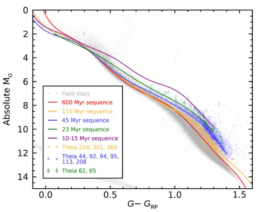
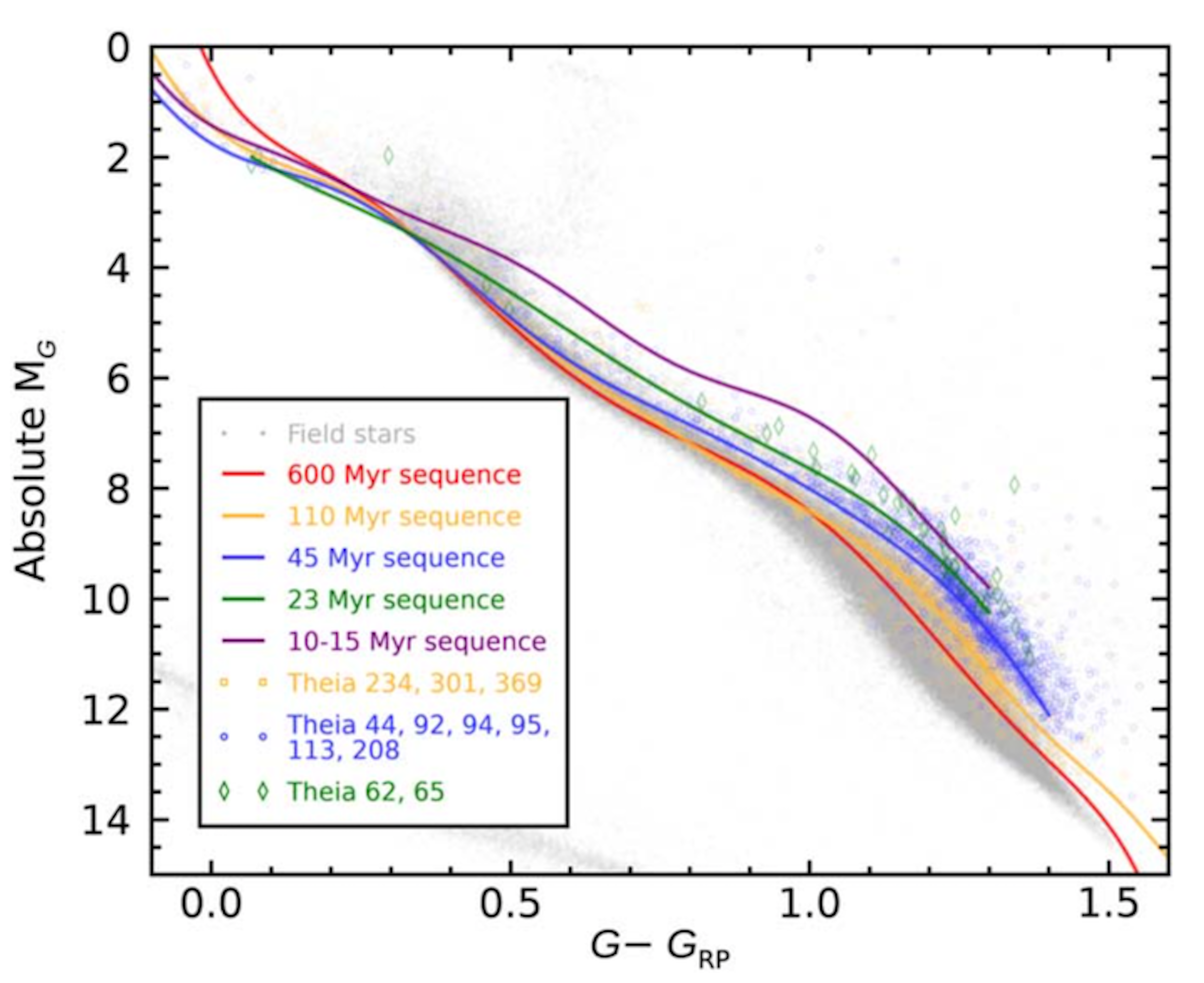
A color–magnitude diagram showing the color of the star against its brightness. The different colors of lines show clusters with different ages. By plotting the new clusters on this map, the team could pinpoint the age of each Theia group. [Gagné et al. 2021]
The team focused on the so-called Theia groups, a large set of stellar structures recently identified within a distance of 10,000 light-years. To determine whether these new stars belong to known groups, the team needed to get a better estimate of their ages. To do this, the authors used data from the Gaia Data Release 2, which was specifically designed to find stars traveling together by measuring their position and how fast they are moving through space.
By using reference stars from five groups of different known ages, Gagné and collaborators fit each Theia group on a color-magnitude diagram, which plots brightness against color. Because the known clusters follow certain trends, placing the new groups on the diagram allowed the authors to find which cluster, if any, the Theia groups were associated with. From this, the authors could estimate how old the groups are.
Sorting into Categories
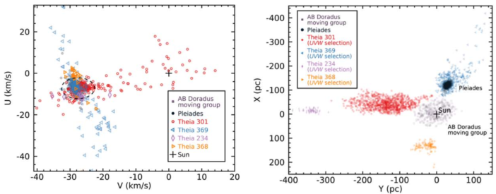
An example of how the team plotted their data for the Pleiades system. Left: the spatial extent of various groups compared to the Pleiades, showing Theia 369 is likely to be associated with it. Right: the velocities of the various clusters. This shows that Theia 369 contains members of the Pleiades and Theia 301 may constitute its trailing tail. [Adapted from Gagné et al. 2021]
When presented with a group of toy cars, a child might sort them by model and color. In the case of Gagné and collaborators’ stellar clusters, once their ages were determined, the team sorted them by how fast they are moving and their sky location. The authors plotted the velocities and spatial distributions of both the Theia groups and known structures, and they found that many of the moving groups and Theia structures are extensions of larger associations of stars or open clusters. This means that these groups are more extended than previously thought, and some might consist of tails that are co-moving with the cores of these clusters.
Some groups may have similar velocities but aren’t physically close to each other, such as Theia 301, which may be extensions of current clusters. For example, Theia 301 and AB Doradus may be trailing tidal tails of the Pleiades. Additional data from Gaia and other missions will provide better constraints on velocities and ages so these groups can properly be sorted where they belong!
Citation
“A Number of Nearby Moving Groups May Be Fragments of Dissolving Open Clusters,” Jonathan Gagné et al 2021 ApJL 915 L29. doi:10.3847/2041-8213/ac0e9a