Features RSS

photograph of an asteroid meteorite sitting on ice

Astronomers wait years for robotic explorers to bring back samples of asteroids — but sometimes, asteroids come to us. What can the meteorites that rain down on Earth tell us about their parent asteroids?

Bringing Outer Space Down to Earth

photograph of a person in the desert with a meteorite

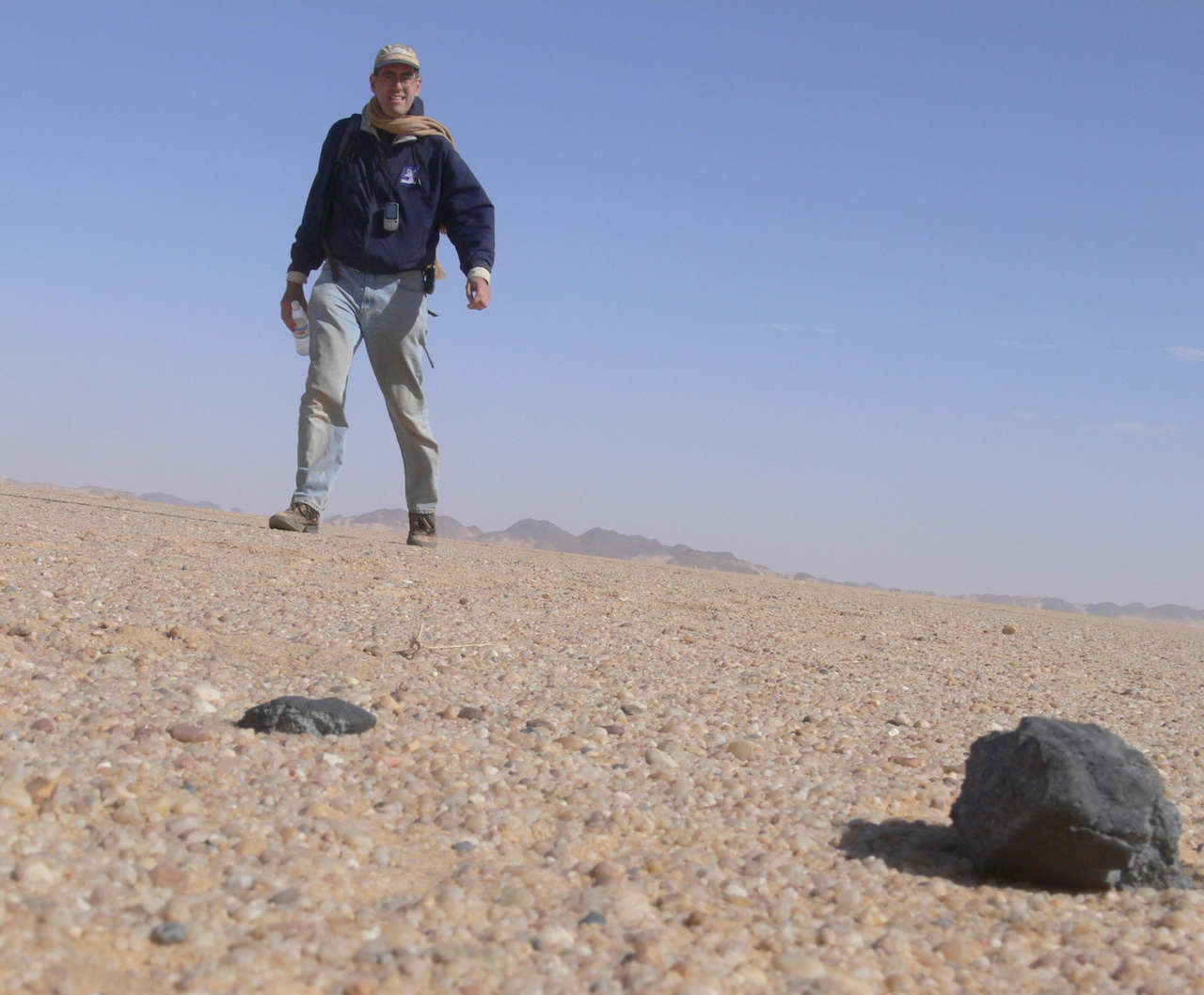
NASA scientist Peter Jenniskens spies an asteroid meteorite in the Nubian Desert in Sudan. The vast majority of meteorites are found in deserts, including Antarctica. [NASA/SETI/P. Jenniskens]

When chunks of asteroids fall to Earth’s surface as meteorites, astronomers seize the opportunity to investigate these remnants of the early solar system. Especially interesting are meteorites called carbonaceous chondrites, which make up less than 5% of all meteorites collected on Earth. Abundance studies suggest that Earth likely accreted many carbonaceous chondrites during its formation, meaning that these meteorites may have been an important source of volatile materials like hydrogen and nitrogen.

In a new article, a team led by Wataru Fujiya (Ibaraki University, Japan) analyzed a slice of the Jbilet Winselwan meteorite, a 6-kilogram carbonaceous chondrite found in Western Sahara in 2013. The team performed laboratory tests to determine the age and composition of the meteorite, as well as what minerals are present, providing clues as to the history of its parent asteroid.

photograph of a sliced meteorite

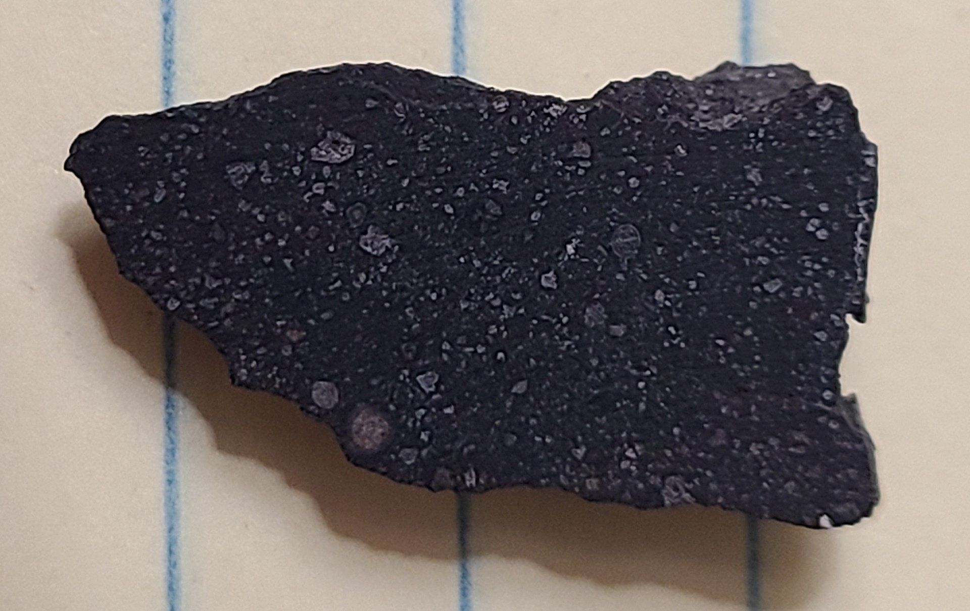
A sliced fragment of the Jbilet Winselwan meteorite. [MJCato; CC BY-SA 4.0]

A Slice of Early Solar System Life

Fujiya and collaborators found that the meteorite contains calcite — a crystalline form of the main component of eggshells, pearls, and chalk — which forms only in the presence of liquid water. Using radioactive dating, the team determined that the calcite in their sample likely formed just 2.6 million years after the solar system formed, meaning that at that point in time, the parent asteroid was warm enough for ice to melt into a liquid.

In fact, the team found signs that the asteroid warmed up far beyond 0°C; some of the minerals had decomposed, which laboratory tests suggest happens at temperatures above 300°C. Space is much chillier than that — what heated this asteroid so quickly after the solar system’s formation?

Sun-Warmed Asteroids, or Something Else?

Modeled thermal history of the meteorite’s parent asteroid. The black and white lines mark temperatures of 0°C and 70°C, respectively. Note that the color scale in the figure gives the temperature in kelvin. [Fujiya et al. 2022]

The authors identified three possible heat sources: solar radiation, impacts by other asteroids, and the decay of radioactive materials. Given the rapid formation of the calcite crystals, the authors concluded that radioactive decay is the most likely heat source for this asteroid; impact heating and solar heating occur intermittently or slowly over billions of years, while radioactive materials churn out heat for just a few million years.

As a test, Fujiya and collaborators modeled the thermal evolution of an asteroid heated by the decay of a radioactive form of aluminum. They found that 20% of the asteroid reached 300°C — hot enough to cause the mineral decomposition seen in the Jbilet Winselwan meteorite.

Additionally, their model showed that while the inner regions of the asteroid were warm enough to have liquid water 0.3 million years after formation, the exterior regions remained cool for a further 0.3–1.0 million years. This explains how dissimilar meteorites could arise from the same asteroid; the Jbilet Winselwan meteorite likely arose from the interior of its parent asteroid, while meteorites that are chemically similar but lack signs of heating might come from the exteriors of asteroids.

Citation

“Hydrothermal Activities on C-Complex Asteroids Induced by Radioactivity,” Wataru Fujiya et al 2022 ApJL 924 L16. doi:10.3847/2041-8213/ac448f

Solid neutron star emitting a burst of radiation

We’re used to watching magnetars throw temper tantrums which involve large outbursts of energy in the form of X-rays. One magnetar, however, recently exhibited some unusual behavior during such an outburst. What’s causing this strange demeanor? 

Whoa, Magnets. 

When it comes to extreme objects in the universe, it doesn’t get more extreme than a magnetar. Take a massive star’s core, crush it into the size of a small city, spin it as fast as a blender, and give it a magnetic field a trillion times Earth’s, and you have yourself a magnetar. The magnetic fields of magnetars are highly complex, and disturbances in these magnetic fields can output vast amounts of energy in the form of X-rays over the span of months or years. A team led by George Younes from the Goddard Space Flight Center / Universities Space Research Association has now monitored a particularly misbehaving magnetar: one that, during such an outburst, changed its behavior in a way that no other magnetar has before. 

Temporal evolution of the pulse profile, showing 3 components on top that morph into one at the bottom

The profile evolution of the magnetar with time with the earliest profile is shown on the top. The vertical lines show the original center of each of the components. [Younes et al. 2022]

A Swift Discovery  

Magnetar SGR 1830-0645 was discovered in late 2020 by the Swift/Burst Array Telescope, a highly sensitive instrument that can pinpoint a burst within seconds of its discovery, after it released a short X-ray burst. It seemed like a normal magnetar with a rotation period of ~10 seconds and a magnetic field strength of ~1014 G (for reference, the magnetic field of Earth is ~0.5 G and the magnetic field of our Sun is ~1 G). While monitoring this energetic event, astronomers noted something odd: this magnetar’s thermal pulse profile, which shows the thermal energy emitted throughout each rotation of the star, gradually changed from having three peaks to having only one. Changes in profile structure have been seen before in magnetars, but the profiles usually get more complex instead of simplifying…so what’s going on?

Crustal Cracking or Magnetospheric Meandering? 

The team observed the source during the first 37 days of the outburst using the Neutron star Interior Composition Explorer (NICER) instrument. They found that the temperature of the star didn’t change, yet the hotspots on the surface (where the emission is thought to come from) get smaller during the outburst. This points to one of two things: either crustal motions or a twisting of the magnetosphere.

Small array of detectors on a rectangular panel mounted on the International Space Station.

The NICER instrument aboard the International Space Station. [NASA]

In the case of crustal motions, magnetic stresses build up under the magnetar’s crust, shifting it much like how tectonic plate motions cause earthquakes. This could cause changes in the active regions where the emission is generated (and, as a bonus, observations of this effect could also tell us about the density of the magnetar’s interior, which is still a bit of a mystery). In the other case, the magnetic field lines in the magnetosphere get twisted and when they untwist, a burst of energy is released (think of a rubber band: when it gets tightly twisted and then let go of, it releases a bunch of energy). It’s also likely that these two mechanisms could both be correct and both be happening at the same time.

Was SGR 1830-0645’s odd behavior during its outburst a one-off event where two mechanisms both happened to come together, or is this common behavior that’s only now detectable due to the NICER instrument’s high-cadence observations? More magnetar observations will tell! 

Citation 

“Pulse Peak Migration during the Outburst Decay of the Magnetar SGR 1830-0645: Crustal Motion and Magnetospheric Untwisting,” George Younes et al 2022 ApJL 924 L27. doi:10.3847/2041-8213/ac4700 

infrared image of the stars and protostars in the orion nebula

photograph of the constellation orion

Visible-light image of the constellation Orion and the Orion nebula — located below the three stars of the “belt” — which is part of the Orion molecular cloud complex. [Wikipedia]

Many mature stars have stellar companions, living out their lives in close-knit clusters or swinging through space in binary pairs. This suggests that most stars form in small groups, but the onset of star formation has long been difficult to study. Now, astronomers have turned arrays of sensitive radio telescopes toward one of the most active star-forming regions in the Milky Way to investigate star formation at its earliest stages.

Star Formation in Our Backyard

When it comes to studying young stars, there’s no better place than the Orion molecular cloud complex: a network of active star-forming regions located just over a thousand light-years away. The Orion molecular clouds contain hundreds of protostars still siphoning gas from their nascent nebulae, making it a perfect arena for studying star formation.

The two leading theories for how stars form are disk fragmentation and turbulent fragmentation. The disk fragmentation theory suggests that a rotating disk of star-forming material can splinter into multiple stars. The turbulent fragmentation theory posits that small fluctuations within a dense clump of gas can ripple outward and induce a gas cloud to collapse. Key to distinguishing between these hypotheses are their length scales; disk fragmentation is thought to produce stars separated by roughly 100 au, while turbulent fragmentation likely generates more widely separated companions.

A First Look at New Stars

Studying star formation at small spatial scales is challenging, because short-wavelength light emitted by young stars is heavily obscured by gas and dust, and long-wavelength observations are inherently lower in resolution. Luckily, the advent of radio telescope arrays has increased the achievable resolution of radio images and allowed astronomers to probe smaller scales than ever before. A team led by John Tobin (National Radio Astronomy Observatory) has used the Atacama Large Millimeter/submillimeter Array (ALMA) and the Very Large Array (VLA) to investigate stellar companionship in the Orion molecular clouds at the earliest stages of star formation — and to explore what these findings mean for how stars form.

plots of radio flux from protostars

Example of observations from ALMA (left) and the VLA (right) of a young protostellar system. [Adapted from Tobin et al. 2022]

Tobin and collaborators surveyed 328 protostars in the Orion molecular clouds, including 94 in the earliest phase of protostar evolution. The team used an iterative algorithm to search for protostars with companions within 20–10,000 au. (For context, if the Sun had a companion at 10,000 au, it would be located in our solar system’s Oort cloud.) The authors found that roughly 30% of all systems surveyed contained multiple stars, with binary systems being more common than triple- or quadruple-star systems.

Competing Creation Scenarios

plot of fraction of companion protostars observed in orion as a function of separation in astronomical units

Separation distribution for multiple-star systems containing the youngest (Class 0) protostars. The dotted curve approximates the distribution for Sun-like stars in the field. [Adapted from Tobin et al. 2022]

The authors noted that the companion separation distribution for the youngest protostars has two peaks — one around 100 au and another around 3,000 au. This suggests that multiple formation mechanisms are at play in these systems; stars that form at large (>500 au) separations via turbulent fragmentation can migrate inward over time, but comparisons with simulations suggest that there are more close-in protostellar companions than can be accounted for by this migration.

The team concluded that more than half of all companions within 500 au likely formed through disk fragmentation, while those at larger separations likely only formed due to turbulent fragmentation. Hopefully, future studies of this rich protostar data set will reveal even more insights about star formation!

Citation

“The VLA/ALMA Nascent Disk And Multiplicity (VANDAM) Survey of Orion Protostars. V. A Characterization of Protostellar Multiplicity,” John J. Tobin et al 2022 ApJ 925 39. doi:10.3847/1538-4357/ac36d2

illustration of a quasar

Supermassive black holes power the bright nuclei of young galaxies in the early universe — quasars. But how do these black holes gain supermassive status in less than a billion years?

Supermassive Centers

simulation of galaxies during the epoch of reionization in the early universe

Simulation of galaxies ionizing hydrogen gas (bright areas) during the epoch of reionization. [M. Alvarez (http://www.cita.utoronto.ca/~malvarez), R. Kaehler, and T. Abel/ESO; CC BY 4.0]

Quasars are truly superlative objects — they are the brightest objects we know of, and some astronomers claim that they’re also the most interesting! Quasars are so luminous that we can observe them at outrageous distances — the most distant quasar discovered shines from roughly 13 billion light-years away. This vast distance means that we see quasars as they were when the universe was less than a billion years old, on the edge of the epoch of reionization, when the first stars and galaxies suffused the universe with photons and put an end to the cosmic dark ages.

These ultra-bright objects are thought to be the nuclei of young galaxies, powered by the accretion of material onto a central supermassive black hole. The presence of supermassive black holes so early in the universe’s history poses a challenge for theorists. How, exactly, does a black hole amass so much material in just a few hundred million years?

plot of absolute magnitude versus redshift

Redshifts and absolute magnitudes of the quasars in this study compared to other studies. Higher redshifts correspond to larger distances and farther back in time. [Yang et al. 2021]

Sensitive Spectroscopy

The size of a supermassive black hole in the early universe is determined by the masses of the smaller black hole “seeds” from which it forms as well as the rate at which it accretes gas from its surroundings. In order to determine the masses and accretion rates of young supermassive black holes, a team led by Jinyi Yang (Steward Observatory, University of Arizona) analyzed infrared spectra of 37 quasars with redshifts between 6.3 and 7.64 — roughly 700 to 900 million years after the Big Bang.

Yang and collaborators calculated the masses of the black holes in their sample to be in the range of 300 million to 3.6 billion solar masses and found that they accrete at 0.26 to 2.3 times the Eddington limit — the theorized point at which the outward push of radiation generated by accretion is so strong that it balances the inward pull of gravity.

Gauging Growth

black hole redshift versus mass

Measured black hole masses (red squares) with black hole growth tracks for different seed masses and accretion rates. [Yang et al. 2021]

The authors estimate that the black holes in their sample must have arisen from black hole seeds no smaller than 1,000 to 10,000 solar masses — but it’s not clear what process could generate these seeds. The collapse of the first generation of stars is one possibility, but these massive stars likely only formed black holes of a few hundred solar masses. Another option is the collapse of gas clouds directly into black holes without first forming stars, but this process is thought to be extremely rare.

Even if the seeds are small, rapid accretion could still bulk these early-universe black holes up to the masses we observe. However, in order to reach billions of solar masses, early-universe black holes would need nearly a billion years of sustained accretion at a rate far exceeding the Eddington limit — anywhere from a few to a few thousand times this limit, depending on the seed mass — and most of the quasars in this study are accreting too slowly. The jury is still out on how supermassive black holes in the early universe gain their impressive size — perhaps in addition to being the most luminous and most interesting objects in the universe, quasars are also the most mysterious!

Citation

“Probing Early Supermassive Black Hole Growth and Quasar Evolution with Near-infrared Spectroscopy of 37 Reionization-era Quasars at 6.3 < z ≤ 7.64,” Jinyi Yang et al 2021 ApJ 923 262. doi:10.3847/1538-4357/ac2b32

photograph of a dusty arm of the milky way galaxy

Did you know that the Sun has a twin? Actually, it has a lot of them — solar twins are born all across the Milky Way. What can we learn about the chemical evolution of our galaxy from these stellar lookalikes?

Familiar Stars

Periodic table of elements showing the likely origin of each element

Periodic table showing the origin of each chemical element. Those produced by the r-process are shaded orange and attributed to supernovae in this image; though supernovae are one proposed source of r-process elements, an alternative source is the merger of two neutron stars. [Cmglee, CC BY-SA 3.0]

The solar neighborhood is populated with stars that have similar temperatures, masses, and radii to the Sun. Though solar twins may seem identical, they vary in a few key ways: they have different ages, they were born at varying distances from the galactic center, and they contain different amounts of heavy elements. Because solar twins span a wide range of ages, astronomers can study them to understand how chemical abundances in the Milky Way have changed over time.

In particular, solar twins provide a way to study elements that form mainly through the r-process: the rapid capture of multiple neutrons in a hot, dense environment. It’s not yet clear where these elements form — core-collapse supernovae were an early contender, but some astronomers now believe that neutron star mergers are the major source of these elements. These two processes differ greatly in their timescales: supernovae could generate r-process elements in just a few million years, while neutron star mergers would likely require billions of years. By tracking the abundances of r-process elements over cosmic time, astronomers can estimate how quickly these elements form — and what produces them.

three plots of elemental abundances of solar twins

Elemental abundances of solar twins in three age groups. Abundances are reported as the log of the ratio with respect to iron (e.g., if X/Fe = 10, [X/Fe] = 1.0). The green bars in the top panel show abundances measured in galactic bulge stars; the correlation suggests that the oldest solar twins originated in the bulge. [Tsujimoto 2021]

Heavy-Metal Patterns Revealed

In order to search for signs of r-process enrichment, Takuji Tsujimoto (National Astronomical Observatory of Japan) analyzed the elemental abundances of 79 solar twins with ages ranging from just 700 million years to 8.7 billion years. Tsujimoto measured the abundances of 28 elements — as light as carbon and as heavy as dysprosium — and found that solar twins of the same age showed the same chemical abundance patterns, but those patterns varied between different age groups.

Both the youngest and oldest solar twins showed signs of enhanced r-process elements compared to iron, while the middle-aged solar twins do not show this intriguing abundance pattern. What does this imply about the sources of r-process elements?

A Resurgent Source

To understand this pattern, Tsujimoto modeled the abundance of europium — an element produced almost exclusively through the r-process — as a function of time. Tsujimoto found that a two-population model was necessary to reproduce the abundance patterns seen in the data, meaning that there are likely two important sources of r-process elements — one that proceeds quickly, leading to enhanced abundances in the oldest twins, and one that proceeds slowly, leading to enhanced abundances in the youngest twins.

plot of europium abundance over time for models and the solar twins studied here

Modeled and observed (gray crosses) europium abundances. [Tsujimoto 2021]

Tsujimoto found that a fast process like supernovae must play an important role in producing r-process elements, though a solely neutron-star origin isn’t out of the question; recently, models have predicted that a subset of neutron star binaries could merge in less than a billion years. For now, the mystery of the origin of r-process elements remains unsolved, though future investigations of distant neutron star mergers may crack the case.

Citation

“Two Sites of r-process Production Assessed on the Basis of the Age-tagged Abundances of Solar Twins,” Takuji Tsujimoto 2021 ApJL 920 L32. doi:10.3847/2041-8213/ac2c75

simulation of gravitational waves from merging black holes

How do binary black holes form? Are the two components born together as stars, or do they find each other only after evolving into black holes? Gravitational waves may hold the answer.

Imprints of Formation History

Gravitational-wave detectors like the Laser Interferometer Gravitational-Wave Observatory (LIGO) and the Virgo interferometer have allowed us to eavesdrop on the mergers of black holes across the universe. With dozens of black hole mergers detected so far, we can start to question how two black holes end up in a binary system in the first place.

Two main pathways are expected. In the first scenario, two stars, coupled since their formation, engage in a slow gravitational dance over billions of years as they evolve into black holes, grow closer, and merge. In the second scenario, two black holes, born apart, become gravitationally entangled in a dynamic environment like a dense star cluster.

gravitational wave forms

An idealized example of gravitational wave forms for a binary black hole system with perfectly circular orbits (e=0; black) and very elongated orbits (e=0.5; red). Click to enlarge. [Abbott et al. 2019]

These two formation pathways affect how eccentric, or elongated, the orbits of the black hole binary pair will be in the moments before they merge. In the isolated origin scenario, the black holes emit gravitational waves as they slowly slink toward each other, leading their orbits to become circular before they merge. In the dynamic origin scenario, on the other hand, black holes that become entangled are driven to merge quickly, before their orbits can circularize. The eccentricity of the binary system alters the gravitational waves released just before the merger, giving astronomers a way to track down the origins of these systems.

eccentricity probability distributions for black hole binaries

Violin plot showing probability distributions for the eccentricities of the 26 binary black hole mergers analyzed in this study and 10 mergers that were previously analyzed. The wider the violin, the more likely the eccentricity. Most events are weighted toward e=0, though two events (GW190620A and GW190521A) show clear signs of nonzero eccentricity. Click to enlarge. [Romero-Shaw et al. 2021]

Examining Eccentricity

A team led by Isobel Romero-Shaw (Monash University and ARC Center of Excellence for Gravitational Wave Discovery, Australia) performed a statistical analysis of gravitational-wave signals from 26 binary black hole mergers in the LIGO/Virgo catalog to determine the most likely eccentricity — and therefore the most likely origin — for each merging system.

Romero-Shaw and collaborators found that while the majority of the events analyzed likely had circular orbits, two events showed clear signs of eccentricity, with 50% of their probability distributions falling above an eccentricity of 0.05. The team’s results suggest that 27% or more of the binary black holes in the LIGO/Virgo catalog formed dynamically, likely in a dense cluster environment.

Emerging Possibilities

ground-based image of a star cluster

Black hole binaries formed in young star clusters, like NGC 3293 shown here, may resemble those formed in dense clusters or isolated environments. [ESO/G. Beccari; CC BY 4.0]

Aside from the systems that were clearly eccentric, Romero-Shaw and collaborators found a further 10 events that showed hints of eccentricity but were still consistent with circular orbits. It’s not yet clear what these marginal detections mean, since random fluctuations could cause perfectly circular binaries to appear eccentric. If these marginal cases truly are eccentric, dense star clusters may not be sufficient to produce the number of observed dynamically assembled systems. This may mean that eccentric black hole binaries can form in other places, such as young open star clusters, which might serve as a gravitational middle ground between dynamic and isolated environments, or the disks surrounding active galactic nuclei.

There’s still much to learn about merging black holes, and luckily our gravitational-wave detectors are hard at work. Hopefully, future detections of black hole mergers help us discern how these systems form!

Citation

“Signs of Eccentricity in Two Gravitational-wave Signals May Indicate a Subpopulation of Dynamically Assembled Binary Black Holes,” Isobel Romero-Shaw et al 2021 ApJL 921 L31. doi:10.3847/2041-8213/ac3138

Pulsar and a larger star

Particles are accelerated all over the universe, but exactly how they get so energetic often remains a mystery. A team of scientists has come up with a model involving stellar winds to explain some intense bursts from binary systems.  

LHAASOing High-Energy Particles

High-energy blasts of radiation can come from all different types of sources, from streams of charged particles from supermassive black holes to high-energy rays produced by our own Sun. Some sources of especially high-energy photons — energetic gamma rays — also produce accompanying bursts of neutrinos.  

Image showing how the IceCube detector works

A diagram of the IceCube detector. [IceCube Collaboration] 

Gamma-ray observatories such as the Large High Altitude Air Shower Observatory (LHAASO) and the Carpet-2 experiment have captured phenomenally energetic photons from more than a dozen sources in the past ten years. Some of these detections have been accompanied by neutrino outflows, which have been observed by the IceCube detector, an observatory at the South Pole containing thousands of sensors distributed throughout a cubic kilometer of Antarctic ice. These detections point to astronomical sources able to accelerate particles to mind-boggling petaelectronvolt (PeV) energies. One PeV is one quadrillion electronvolts — one thousand times the kinetic energy of a flying mosquito, packed into a single particle. A group led by Andrei Bykov from the Ioffe Physical-Technical Institute in Russia may have now come up with a model to explain what powers these ultra-energetic accelerators. 

A Compact Explanation 

A diagram of the Be star and complex object, showing how the winds collide to accelerate particles.

A diagram of the model. The pulsar wind is in pink, the cross-hatched green is the zone of contact discontinuity, the blue is the stellar wind. [Bykov et al. 2021]

The authors’ model involves a binary system consisting of a Be star — a B spectral giant that emits Balmer lines in its emission — and some type of compact object. The two objects each have a stellar wind, and the collision of those stellar winds accelerates protons up to the PeV range. From there, the protons collide with photons to produce PeV-regime gamma rays and neutrinos. This model allows a large fraction of the kinetic energy of the outflows of compact object binary systems to be converted into energy in the PeV range and provides a high flux of neutrinos. 

This scheme explains how these events get so energetic, and it can even explain lower-energy gamma-ray events that coincide with high-energy neutrinos. These neutrinos, which may greatly contribute to the high-energy neutrino flux in the galaxy, should be detectable by IceCube, so future observations may provide a test of this model. 

Citation 

“PeV Photon and Neutrino Flares from Galactic Gamma-Ray Binaries,” A. M. Bykov et al 2021 ApJL 921 L10. doi:10.3847/2041-8213/ac2f3d 

artist's impression of a pulsar

Does Einstein’s general theory of relativity stand the test of time, or does this famed description of gravity waver under scrutiny? A team of astronomers has used a pair of ultra-dense stellar remnants to put the theory to the test.

reproduction of a 1919 photograph of the solar corona during a total solar eclipse

An image of the Sun based on a reproduction of a photograph negative created during Sir Arthur Eddington’s 1919 expedition to verify the general theory of relativity. [Frank Watson Dyson]

New Test of an Old Theory

In 1919, scientists journeyed to Brazil and São Tomé and Príncipe to witness a solar eclipse and measure the subtle bending of starlight caused by the Sun’s mass. This experiment was one of the first of a highly publicized series of tests of the general theory of relativity, which governs the warping of spacetime by matter and energy. The theory has withstood test after test, but that hasn’t stopped astronomers from trying to confound it.

As our understanding of the universe and the tools at our disposal have grown more sophisticated, so too have our tests; now, a team led by Hao Ding (Swinburne University of Technology and ARC Center of Excellence for Gravitational Wave Discovery, Australia) has joined the storied quest to probe the century-old theory of gravitation using a type of object not yet known to the world when Einstein penned the theory in 1915 — pulsars.

artist's impression of a pair of pulsars

An artist’s impression of a pair of pulsars. [Michael Kramer (Jodrell Bank Observatory, University of Manchester)]

Tracking a Binary System

Pulsars are highly magnetized, extremely dense stellar remnants that emit beams of radiation. In rare cases, the two stars in a binary system can both evolve into pulsars; the 1974 discovery of a pulsar in a binary system and its importance as a test bed for theories of gravitation won Russell Hulse and Joseph Taylor a Nobel Prize.

Astronomers use binary pulsars to test the predictions of general relativity by measuring the rate at which their orbits decay as they lose energy in the form of gravitational waves. Past measurements of the orbital decay rate for one of the 16 confirmed pulsar binaries, PSR J1537+1155, disagreed with the predictions of relativity by 9% — a far larger discrepancy than has been found for other systems.

A major difficulty of performing this test lies in determining the distance to PSR J1537+1155, which moves across the sky at an unusually quick pace; unfortunately, the best way to measure the distance to a pair of pulsars uses the predictions of general relativity — so it can’t be used in a test of the theory. Now, Ding and collaborators have determined a new distance to PSR J1537+1155 the old-fashioned way: by measuring the system’s apparent motion relative to background stars as Earth moves around the Sun.

Questing for Precision

radio telescope in front of a mountain range

One of the 25-meter radio telescopes in Owens Valley, California, which is one of the 10 sites that make up the VLBA. [NRAO/AUI/NSF; CC BY 4.0]

For their updated distance measurement, Ding and collaborators used data from the Very Long Baseline Array (VLBA) — a network of radio telescopes scattered across the globe with the resolving power of a single 5,351-mile-wide radio dish. The team carefully combined measurements taken over a six-year period to get the most precise distance to a binary pulsar system ever obtained without assuming relativity to be correct: 0.94 kiloparsec (3,066 light-years).

With this new measurement, the disagreement between observations and the predictions of relativity shrinks to just 2.3%. Looking to the future, Ding and collaborators anticipate that high-sensitivity very long baseline interferometry measurements will further refine our estimate of the distance to PSR J1537+1155 and potentially resolve the remaining tension between observations and theory.

Citation

“The Orbital-decay Test of General Relativity to the 2% Level with 6 yr VLBA Astrometry of the Double Neutron Star PSR J1537+1155,” Hao Ding et al 2021 ApJL 921 L19. doi:10.3847/2041-8213/ac3091

image of the sun's surface

Sophisticated machine-learning techniques may finally answer a question astronomers have pondered for decades: what makes the Sun launch solar flares?

Predicting and Pattern-Finding

extreme-ultraviolet image of the sun with a magnetic field model overlaid

Why study the causes of solar flares? Flares are just one example of how the Sun’s complex magnetic field interacts with its dynamic plasma environment. [NASA/GSFC/Solar Dynamics Observatory]

In recent years, researchers have explored using machine learning to understand the causes of solar outbursts like solar flares and predict their onset. Computers excel at sifting through mountains of data and finding subtle patterns that would elude a manual search. After these patterns have been dredged up, researchers can interpret and model them, yielding new insights. This process may not only help predict solar flares before they happen, but it also might help us understand the physical mechanism that launches these powerful events and gain a better understanding of the complex plasma environment of the Sun’s atmosphere.

In a new study, a team led by Magnus Woods (Bay Area Environmental Research Institute and Lockheed Martin Solar and Astrophysics Lab) applied a machine-learning algorithm to ultraviolet solar spectra to identify signs that a solar flare is imminent — should any such signs exist.

image of the sun

A sample image of the Sun from IRIS, showing twisting structures dubbed “mini-tornadoes.” [NASA/IRIS/Pereira]

Spectral Signatures of Future Flares

Woods and collaborators used spectra from the Interface Region Imaging Spectrograph (IRIS) — an Earth-orbiting spacecraft dedicated to understanding the region of the Sun’s atmosphere in which the temperature increases sharply from a few thousand kelvin to millions of kelvin. The team selected three sets of observations for analysis: quiet Sun (no areas of enhanced magnetic fields), quiescent active region (enhanced magnetic fields but no solar flares), and flares. By comparing observations known to contain solar flares to those without, the team aimed to narrow in on spectral features that are uniquely associated with flares.

The team focused on the magnesium h and k lines, which are prominent features in the wavelength range monitored by IRIS. Their machine-learning technique pinpointed interesting behavior in these spectral lines; typically, the h and k lines are double peaked, but under the conditions that precede a solar flare — up to 40 minutes in advance — they retain only a single peak.

More To Learn

spectral lines of magnesium

The two types of spectral signatures associated with pre-flare conditions. Individual profiles are in black and a representative profile is in orange. The data are reported in counts per second. [Adapted from Woods et al. 2021]

Woods and collaborators found that the single-peaked magnesium lines also appeared in quiescent active regions, but they were far more prevalent in the pre-flare regions. The quiescent active regions with single-peaked spectral lines also exhibited small-scale brightening events — not full-on solar flares, but further evidence that this spectral feature is associated with solar heating.

The team determined that the observed spectral features were associated with rising temperatures roughly 1,000 kilometers above the Sun’s surface. This suggests that the warning signs of solar flares are generated in this region, though more work is needed to confirm this result. The enormous wealth of solar spectral and magnetic data makes teasing out the fleeting signatures of solar flares a tall order, but this work makes it clear that machine learning can bring us a step closer to understanding the causes of solar flares.

Citation

“Unsupervised Machine Learning for the Identification of Preflare Spectroscopic Signatures,” Magnus M. Woods et al 2021 ApJ 922 137. doi:10.3847/1538-4357/ac2667

multiwavelength image of supernova remnant IC 443

Sometimes, the properties of massive astrophysical objects are determined by some of their smallest components: electrons. Today’s article explores an intriguing idea: what if the differences between some mysterious explosions across our universe can be explained by the behavior of electrons?

image of AT2018cow's location

Image from the Sloan Digital Sky Survey with cross hairs pinpointing the location of AT2018cow. It is spatially coincident with the galaxy CGCG 137-068 in the constellation Hercules. [Sloan Digital Sky Survey; CC BY 4.0]

New Kid in the Universe

In 2018, a telescope searching for near-Earth asteroids witnessed a fleeting explosion nearly 100 times more luminous than a typical supernova in a galaxy 200 million light-years distant. The event — dubbed AT2018cow — was the first of a new class of phenomena called fast blue optical transients. Astronomers have yet to agree on the cause of these rare events, but many explanations center on an exploding object that expands into surrounding gas.

These mysterious new transients aren’t the only astronomical example of explosions colliding with nearby material; supernovae that emit strongly at radio wavelengths — aptly named radio supernovae — arise when an expanding shock wave plows into circumstellar gas. However, their spectra are very different from those of fast blue optical transients. Are radio supernovae and AT2018cow-like events completely unrelated, or could a common thread tie them together?

Shocking Similarities

spectral energy distributions

Example spectral energy distributions showing peak emission dominated by thermal electrons (top) and non-thermal electrons bottom). [Adapted from Margalit & Quataert 2021]

Picture this: millions of light-years away, there’s an explosion. Maybe it’s a garden-variety supernova, or maybe it’s something far stranger. Either way, the explosion launches a shock wave that sweeps up material and accelerates electrons to relativistic speeds. Typically, astronomers assume that many of these shock-accelerated electrons are zipping around faster than they would be if they were all in thermal equilibrium. This non-thermal electron model can explain the emission from radio supernovae, but it can’t explain rare transient events like AT2018cow. Recently, researchers modeled a population of thermal electrons instead and were able to reproduce the emission of an AT2018cow-like event.

This suggests that seemingly disparate phenomena like radio supernovae and AT2018cow-like events could both be explained by the shock-accelerated electron model — just by tweaking a few properties of the electrons. In a new study, Ben Margalit (University of California, Berkeley) and Eliot Quataert (Princeton University) modeled the emission from a mixture of thermal and non-thermal electrons to explore how different electron behaviors affect the emission we observe.

Varied Outcomes

Margalit and Quataert found that thermal electrons are critical for modeling some — but not all! — shock waves, and whether or not thermal electrons are important is mainly determined by the speed of the shock. For example, shocks that move relatively slowly, like those seen in radio supernovae, show virtually no emission from thermal electrons. As a result, a solely non-thermal electron model can reproduce those events. For AT2018cow-like events, where the shock moves at a substantial fraction of the speed of light, including thermal electrons is critical for reproducing their spectra. The authors found that including a thermal electron component becomes necessary when modeling shocks moving faster than 20% the speed of light.

illustration of the aftermath of two neutron stars merging

The collision of two neutron stars, illustrated here, may be a target for the authors’ model. [NASA Goddard Space Flight Center/CI Lab]

Although this work is motivated by observations of radio supernovae and AT2018cow-like events, the authors note that their model should apply to other astrophysical blasts, such as shock waves produced by colliding neutron stars or fading gamma ray-bursts. Future modeling of these and other events may further highlight role that humble electrons play in influencing the appearance of explosions in our universe.


Citation

“Thermal Electrons in Mildly Relativistic Synchrotron Blast Waves,” Ben Margalit and Eliot Quataert 2021 ApJL 923 L14. doi:10.3847/2041-8213/ac3d97

1 46 47 48 49 50 119