Features RSS

Three side by side images with the same galaxy in the center. In the center panel, a supernova is visible to the right of the galaxy.

Why did a supernova observed back in 2021 initially emit so much ultraviolet light, then abruptly shift color? A recent study suggests a change in ejecta velocity, a cosmic speed bump, may be the culprit.

Brief Flashes

If you want to study the moments after a white dwarf explodes, speed is key. Each view of these violent ends, dubbed Type Ia supernovae, is temporary: we see a point of light grow brighter, then fainter over the course of months, and many of the interesting science questions can only be answered by catching the earliest moments after the eruption. This is an extremely difficult task considering that no one knows where a Type Ia supernova might go off, and consequently astronomers must scan the entire sky looking for tiny pinpricks of light that weren’t there before.

Although the adoption of automated telescopes in recent years has made this continuous needle-in-a-haystack search easier, it is still rare for astronomers to collect thorough measurements of a supernova many days before it reaches peak brightness. Recently, however, a team led by Chris Ashall (University of Hawaiʻi at Manoa) did just that, and what they found was somewhat surprising.

Too Blue

A two panel plot, both showing time on the x. The bottom panel y axis is B-V color, and the top panel y axis is normalized flux.

Top: the u-band photometry of SN 2021aefx measured in days until peak brightness, along with several possible fits. Bottom: the color evolution of SN 2021aefx, which reverses direction about 16 days before maximum brightness. Another supernova that followed a similarly non-monotonic path, SN 2018aoz, is included for comparison. [Adapted from Ashall et al. 2022]

The team’s target, named SN 2021aefx, initially emitted lots of ultraviolet light (u-band light, in observational astronomy parlance). However, in the first days after the explosion as the remnants grew brighter across all wavelengths, the growth of the u-band light didn’t follow the expected t2 power law. Instead, after its strong start, the ultraviolet emission stumbled: it still grew brighter, but followed a gentler two-component model with two different power indices. While the u-band emission faltered, all other wavelengths grew as expected, and this relative difference in growth rates changed color of the supernova soon after initial detection.

To figure out why this offbeat supernova generated so much ultraviolet light before changing its tune, the team collected spectra as well as multiband photometry. These data revealed that the supernova ejecta had a very high initial velocity of about 30,000 km/s 17 days before peak brightness, but that it slowed to 21,000 km/s less than two days later.

Slow It Down

A plot of flux vs. wavelength. The initial spectrum is duplicated many times and blueshifted to different amounts to demonstrate that a velocity change could alter the amount of light in the u band. The bandpasses of the u and B bands are shown behind the spectra.

A spectrum of SN 2021aefx taken 17.3 days before maximum brightness, artificially blueshifted by different amounts. The u and B bandpasses are marked in blue and red, respectively. Note on the inset that blueshifts affect the observed flux within the u band, but only weakly affect the B-band values. [Adapted from Ashall et al. 2022]

That speed change, combined with the difference in spectral shape across the u and B bands, was key to the authors’ explanation of the excess ultraviolet light. By artificially adjusting the velocity of their spectrum, Ashall and collaborators demonstrated that they could blueshift their way to a higher u-band measurement without affecting their B-band values. Putting it all together, the team claimed that the guts of this star hit a speed bump: when the ejecta were bolting out of the gate, more of their emitted light fell into the u band, but after abruptly slowing down, their emission tumbled back into the B band.

This study only focused on observations between 17 and 6 days before peak brightness, though the authors plan to publish fuller light curves they acquired. In the meantime, we’ll have to wonder about any other obstacles these supernova remnants might face on their journey through the universe.

Citation

“A Speed Bump: SN 2021aefx Shows that Doppler Shift Alone Can Explain Early Excess Blue Flux in Some Type Ia Supernovae,” C. Ashall et al 2022 ApJL 932 L2. doi:10.3847/2041-8213/ac738c

coronal mass ejection

The Sun launches tangled masses of plasma and magnetic fields in the form of coronal mass ejections. But these explosions don’t occur in a (literal or metaphorical) vacuum — how is the passage of a coronal mass ejection affected by the eruptions that preceded it?

Capturing Coronal Mass Ejections

Illustration of the sun setting off a coronal mass ejection headed to Earth and it hitting Earth's magnetosphere

Illustration of a coronal mass ejection headed toward Earth. [SOHO/LASCO/EIT (ESA & NASA)]

When the Sun’s activity cycle ramps up to its maximum, as it will in 2025, the Sun will unleash two or three coronal mass ejections every day. These explosions blast out into the solar system, speeding toward Earth and the other planets at hundreds of kilometers a second. When a coronal mass ejection collides with Earth’s protective magnetic field, the ensuing magnetic tussle can fling high-energy particles into Earth’s atmosphere, creating the aurora — and potentially damaging spacecraft electronics.

Given the risk of damaging effects on Earth-orbiting spacecraft, researchers have developed models to predict the path a coronal mass ejection will take after detaching from the Sun. These models estimate how a loop of magnetized plasma twists, expands, and is deflected as it travels through the tenuous swirls of the solar wind. However, many such models trade accuracy for speed in order to quickly assess the danger to Earth, failing to capture the variable and turbulent nature of the space between Sun and Earth, which may affect how coronal mass ejections travel through that space.

A Series of Solar Events

A team led by Chin-Chun Wu (Naval Research Laboratory) used magnetohydrodynamics simulations to explore how a coronal mass ejection moves through the wake left by previous solar eruptions. Wu and collaborators opted to model a series of five coronal mass ejections that occurred in two and a half weeks in July 2012, for which we have extensive data.

Modeled radial solar wind speed for four time periods

Modeled radial solar wind speed for four time periods. The red areas indicate coronal mass ejections. Click to enlarge. [Adapted from Wu et al. 2022; full time series available here]

The team’s model uses observations of these events to determine each coronal mass ejection’s initial speed, trajectory, and the time it departs the Sun. By solving fluid dynamics equations to understand how each event evolves over time, the model outputs key parameters like the plasma density and temperature, the speed of the background solar wind, and the magnetic field strength, all of which can be compared against measurements made by satellites.

Creating a Path to Follow

comparison of observed and modeled plasma parameters

Observed (black points) and modeled (red and purple lines) plasma parameters. The model results for a series of three coronal mass ejections are shown as red dotted lines, and the model results for a single coronal mass ejection are shown in purple lines. From top to bottom, the parameters shown are the radial velocity (vr), the plasma density (np), the plasma temperature (Tp), and the magnetic field strength (B). Click to enlarge. [Wu et al. 2022]

Previous work has suggested that when one coronal mass ejection closely follows another, the second event moves faster than it would otherwise. To test this theory, Wu and coauthors compared a model of a series of coronal mass ejections to another of just the final event in the series. These simulations showed that a coronal mass ejection following in the wake of other explosions travels faster than one forging ahead solo — the passage of a previous shock wave reduces the density and increases the speed of the solar wind, allowing the final coronal mass ejection to surf its way to Earth’s orbit 30 minutes faster.

Ultimately, the authors concluded that their model was able to match the observed parameters of the five coronal mass ejections fairly well. Their simulations allowed them to show that coronal mass ejections are affected by those that came before, suggesting that multiple events should be accounted for in modeling these eruptions.

Citation

“Magnetohydrodynamic Simulation of Multiple Coronal Mass Ejections: An Effect of Pre-events,'” Chin-Chun Wu et al 2022 ApJ 935 67. doi:10.3847/1538-4357/ac7f2a

An image of the TW Hydrae disk, zoomed out far enough that the entire disk is visible and a set of concentric dark rings neatly surround the central star.

The gorgeous, nearby, face-on TW Hydrae protoplanetary disk has proved challenging to quantify: just how much gas is sitting between those rings? A new study presents a possible answer and develops a new technique for addressing the question along the way.

Covert Disks

Much like babies cling to their blankets, young stars wrap themselves in disks of gas and dust when they’re very young. Although this state of infancy lasts only a short few million years, this temporary cosmic comforter is a profoundly important artifact of a star’s birth, at least from our earthly perspective. That’s because all planets, asteroids, and humans formed from this material: we are the worn remains of a structure long ago dispersed, clumps of matter that couldn’t get blown away in our Sun’s angsty teenage years when it scattered the rest of its protoplanetary disk.

Basic measurements such as how gas is distributed around young stars are therefore vital for our models of planet formation. Unfortunately, this measurement is notoriously tricky to make since the most dominant component of the disk, hydrogen gas, stubbornly refuses to emit light while at the temperatures in this environment. Most of astronomy relies on catching photons flung our way across the void, but if the hydrogen refuses to play catch, we can’t see it.

An image showing emission from the small region of sky surrounding TW Hydrae. Equal brightness contours appear as concentric rings centered on inner region of the disk.

Emission from dust in the TW Hydrae protoplanetary disk, colored by brightness temperature of the dust. Axes are in arcseconds. [Tsukagoshi et al. 2019, reproduced in Yoshida et al. 2022]

Luckily, although we cannot detect most of the disk, other components besides hydrogen are more amenable to electromagnetic communication. Dust, for example, glows even while embedded in the hydrogen, so we can measure its distribution and use it as a proxy for the gas distribution. However, this method relies on an assumed gas-to-dust ratio and profile, which isn’t always certain. Alternatively, various forms of CO also shine through the gas, but the ratio of CO to hydrogen is likely unique to each disk. As a result of these uncertainties, previous estimates of the total mass of the nearby TW Hydrae disk have spanned more than an order of magnitude.


Pressure Wings

A plot of flux vs. velocity shift. The data is a broad downward-opening V, while the comparison Gaussian profile is a much narrower V. The model closely follows the data.

An illustration of the pressure-broadened wings. The dashed line marks a typically used Gaussian shape, while the green line shows the best-fitting Voigt profile, which captures broadening. The data are shown in black, and the 3-sigma significance level is denoted by the dotted line. [Yoshida et al. 2022]

A new study led by Tomohiro C. Yoshida (National Astronomical Observatory of Japan; The Graduate University for Advanced Studies) develops a workaround to these challenges: rather than relying on a tracer, the team instead looked at the shape of CO lines at the inner region of the disk.

Typically, astronomers assume these lines follow a roughly Gaussian shape. However, Yoshida and collaborators found that in the inner regions of the disk, the “wings” of the lines were wider than expected. After considering various explanations for what might cause this broadening, they concluded that the wings are the result of higher pressures along the midplane of the disk.

This new method should be applicable to other disks moving forward, so astronomers can hope for similarly refined measurements in the near future.

Citation

“Discovery of Line Pressure Broadening and Direct Constraint on Gas Surface Density in a Protoplanetary Disk,” Tomohiro C. Yoshida et al 2022 ApJL 937 L14. doi:10.3847/2041-8213/ac903a

Cassini spacecraft image of the surface of Saturn's moon Enceladus

The icy moons of the outer solar system are a promising place to look for life beyond Earth, and a new research article shows that we already have the tools to start our search.

Biosignature Possibilities

Cassini image of plumes on Enceladus

An image of Enceladus’s water plumes taken by Cassini. The small moon has more than a hundred such geysers. [NASA/JPL/Space Science Institute]

While the search for life beyond Earth often focuses on our neighboring planet Mars or the promise of distant, Earth-like exoplanets, icy moons in our solar system have recently come to the forefront of this discussion. Researchers suspect that many of the moons in the outer solar system have oceans hidden beneath their icy or rocky crusts — and the plumes of water ice observed shooting from fissures in the surface of Saturn’s moon Enceladus may provide an excellent way to study one of these oceans directly.

If life is present in the oceans of Enceladus or other icy moons in the solar system, it’s possible that plumes could deposit life-signaling molecules — biosignatures — on the surfaces of these worlds. A recent publication tests our ability to detect a certain class of biosignature compounds: lipids.

chemical structure of cholecalciferol

The chemical structure of a lipid called cholecalciferol. Cholecalciferol is better known as vitamin D. [Wikipedia user Calvero; Public Domain]

Measuring Samples with Mass Spectrometry

Though the term lipids might not be familiar, the molecules themselves likely are: lipids include fats, waxes, and certain vitamins. Lipids are also important components of cell membranes, making them essential to all life on Earth. Their size and complexity mean they’re unlikely to form through simple chemistry, making them potential biosignatures. But how would we detect these molecules on another world?

Rather than attempt to detect these molecules from afar, we’ll likely need to sample them directly by sending an instrument down to the surface of the planet or moon we want to study. In a recent publication, a team led by Nikita Boeren (University of Bern, Switzerland) tested the abilities of a candidate lipid-detecting spectrometer called the ORganics Information Gathering INstrument (ORIGIN).

ORIGIN is a laser desorption ion mass spectrometer, a type of instrument that uses a pulse of laser light to remove (desorb) molecules from a surface and ionize them. These electrically charged molecules are then channeled toward a detector by electric and magnetic fields, and the time that each molecule takes to reach the detector is related to the ratio of the molecule’s mass to its electrical charge. Using the mass-to-charge ratio of the molecule and any fragments it might have split into, researchers can determine which molecules were present in the sample.

Looking for Lipids

Boeren and collaborators tested ORIGIN’s ability to detect pure samples of six varieties of lipids, as well as combinations of those same lipids with other organic molecules: amino acids (compounds often referred to as “the building blocks of life”) and polycyclic aromatic hydrocarbons (molecules containing rings of carbon atoms).

mass spectra for mixtures of different substances

Mass spectra for a mixture of six lipids (top), four lipids mixed with two amino acids (middle), and four lipids mixed with two polycyclic aromatic hydrocarbons (bottom). Click to enlarge. [Boeren et al. 2022]

The team’s results show that the instrument is capable of detecting and differentiating between several different lipid molecules, even when those substances were mixed with other compounds. While more work remains to be done, including testing the procedure on other lipids and exploring the effects of using different types of materials to hold the sample, ORIGIN already shows great promise as a way to detect biosignature compounds. In fact, the detection limits determined in this study meet the requirements of the Enceladus Orbilander, a high-priority mission proposed in the 2023–2032 Planetary Science Decadal Survey.

Citation

“Detecting Lipids on Planetary Surfaces with Laser Desorption Ionization Mass Spectrometry,” Nikita J. Boeren et al 2022 Planet. Sci. J. 3 241. doi:10.3847/PSJ/ac94bf

Hubble Space Telescope image of SN1987A

Astronomers observe and model exploding stars to understand the details of stellar evolution, map the chemical enrichment of our galaxy, and even estimate the expansion of the universe. Today we take a look at five recent approaches to supernova science, from assessing the behavior of a single star to making plans for future surveys that will detect thousands of supernovae every year.

Radio Investigation of an Exploding Star

observations and models of the radio evolution of SN 2016gkg

Radio spectra observed with the Jansky Very Large Array (circles) and the Giant Metrewave Radio Telescope (squares) compared to best-fitting models (solid lines). [Nayana A. J. et al. 2022]

Nayana A. J. (Indian Institute of Astrophysics) and collaborators monitored the supernova SN 2016gkg for nearly four years, starting just eight days after the initial explosion. Modeling of SN 2016gkg’s optical light curve suggest that it’s a Type IIb supernova, meaning that it resulted from the collapse of a massive (>8–10 solar masses) star that once possessed a hydrogen-rich envelope of material, most of which was lost before the star collapsed.

While it’s possible to identify the star that went supernova in images taken before the explosion, researchers rely on models of supernova light curves to extract details about the material surrounding the star, which can hold clues about the star’s behavior before it went supernova. The team modeled SN 2016gkg’s radio light curves and spectra, simulating the effects of a shock wave plowing into material previously released by the star. The results suggested that the shock wave from SN 2016gkg expanded outward at 10% the speed of light into stellar wind material produced in the last hundred years of the star’s life.

Accounting for Cooling

C.-I. Björnsson (Stockholm University, Sweden) investigated the radio-wavelength behavior of another supernova, SN 2020oi. SN 2020oi is classified as a Type Ic supernova, which means the explosion resulted from the collapse of a massive star that had lost its hydrogen envelope. Type Ic supernovae are distinguished from other types of supernovae by their spectra, which have weak or no spectral features from silicon or helium.

Björnsson modeled the supernova’s radio emission, which is largely produced by electrons traveling in helical paths around magnetic field lines. Where Björnsson’s modeling differs from previous modeling efforts is the inclusion of radiative cooling by these spiraling electrons in the spectral fitting process, rather than assessing the cooling rate after the fitting is done. The author demonstrated that accounting for cooling during the fitting process alters the inferred properties of the event; for example, while previous analyses have invoked a varying pre-explosion mass-loss rate to explain some features of SN 2020oi’s light curve, Björnsson found that incorporating cooling removed the need for a changing mass-loss rate.

derived upper limits on the instrinsic strain for NS 1987A

Upper limits on the intrinsic strain (a dimensionless quantity related to the amplitude of a gravitational wave; shown here in blue points) compared to an indirect limit on the strain set by the conservation of energy. [Adapted from Owen et al. 2022]

A Search for Gravitational Waves

SN1987A is one of the best-studied supernovae, but astronomers are still debating what it left behind. Multiple lines of evidence suggest that the explosion resulted in a neutron star — a city-sized stellar core so compressed that protons and electrons are squished together into neutrons — but the remnant has never been detected directly. Recently, a team led by Benjamin Owen (Texas Tech University) searched for gravitational waves from the purported neutron star. Unlike two objects colliding, which produces a sudden gravitational wave chirp, a young neutron star would emit gravitational waves constantly, powered by the slow spin-down of the rapidly spinning star.

Guided by knowledge of the neutron star’s likely distance, age, and size, the team searched through observations from the Laser Interferometer Gravitational-Wave Observatory (LIGO) but found no signal. However, the search allowed them to place upper limits on the neutron star’s gravitational wave emission and place constraints on the object’s properties, such as its ellipticity and magnetic field strength. As more precise search methods and gravitational wave data become available, Owen and collaborators anticipate more exacting searches will be possible in the future.

Preparing for the Future

Brian Hsu (Center for Astrophysics ∣ Harvard & Smithsonian) and collaborators looked ahead to future surveys, like the Vera C. Rubin Observatory Legacy Survey of Space and Time (LSST), which will produce a vast archive of photometric data. While LSST presents an incredible opportunity to study transient events, including supernovae, it also presents a challenge — how do we use photometric data to identify transient events that normally require spectroscopic data to classify? As an example, the authors considered superluminous core-collapse supernovae, which account for just 0.1% of all core-collapse supernovae but are overrepresented in surveys due to their extreme brightness (10–100 times brighter than a typical supernova).

posterior distributions of magnetar parameters

Posterior distributions of magnetar parameters derived from light curve modeling. Click to enlarge. [Hsu et al. 2022]

Hsu and collaborators used photometric data from the Pan-STARRS1 Medium Deep Survey to train a machine-learning algorithm to identify superluminous supernovae using only photometry. The team fit the light curve for each event with a model representing the spin-down of a magnetar — a neutron star with an extremely strong magnetic field — which is thought to power these events. This allowed them to determine the likely properties of the supernovae in their sample and compare these properties to those of supernovae that were selected spectroscopically. The team found that the two supernova samples had similar properties overall, though the photometrically selected sample captured events driven by magnetars that spun more slowly. While the team noted several challenges related to their technique, they anticipate that machine-learning tools will provide a way to extract valuable insights from the upcoming wealth of photometric data.

Studying Standard (and Over-Luminous) Candles

Not all supernovae are the result of massive stars collapsing; Type Ia supernovae occur when a stellar companion contributes mass to a white dwarf — an Earth-sized stellar core left behind when a low- or intermediate-mass (<8 solar masses) star exhausts its supply of hydrogen and loses its outer layers. All Type Ia supernovae are hypothesized to occur when a white dwarf reaches 1.44 solar masses, resulting in explosions of (theoretically) identical brightness. This makes Type Ia supernovae extremely valuable as standard candles, helping researchers gauge the distances to galaxies and even study the expansion of the universe.

Histogram of absolute magnitude during peak brightness of typical Type Ia supernovae and over-luminous Type Ia supernovae

Histogram of absolute magnitude during peak brightness of typical Type Ia supernovae (black) and over-luminous “91T/99aa-like” Type Ia supernovae (red). [Adapted from Yang et al. 2022]

However, in reality, not all Type Ia supernovae are equally luminous, and understanding how these events differ is critical to calibrating our observations and ensuring that Type Ia supernovae remain useful as standard candles. Jiawen Yang (Texas A&M University) and collaborators used observations of two varieties of Type Ia supernovae — 37 over-luminous Type Ia supernovae and 87 typical ones — to assess the differences between them. The authors found that the over-luminous supernovae are systematically 0.2 magnitude brighter than typical supernovae, even after applying several corrections to their light curves.

Because the two types of supernovae fade similarly in the months after exploding, Yang and collaborators point out that identifying over-luminous supernovae as they approach peak brightness is necessary. Otherwise, these over-luminous supernovae might be mistaken for typical supernovae, biasing calculations of cosmological distances. Accounting for differences in the light curves of Type Ia supernovae will become especially important for interpreting the results of future all-sky surveys, since these surveys will discover an outsize number of over-luminous Type Ia supernovae.

Citation

“Radio Evolution of a Type IIb Supernova SN 2016gkg,” Nayana A. J. et al 2022 ApJ 934 186. doi:10.3847/1538-4357/ac7c1e

“Radio Spectra of SN 2020oi: Effects of Radiative Cooling on the Deduced Source Properties,” C.-I. Björnsson 2022 ApJ 936 98. doi:10.3847/1538-4357/ac87aa

“First Constraining Upper Limits on Gravitational-wave Emission from NS 1987A in SNR 1987A,” Benjamin J. Owen et al 2022 ApJL 935 L7. doi:10.3847/2041-8213/ac84dc

“Photometrically Classified Superluminous Supernovae from the Pan-STARRS1 Medium Deep Survey: A Case Study for Science with Machine-learning-based Classification,” Brian Hsu et al 2022 ApJ 937 13. doi:10.3847/1538-4357/ac87ff

“Using 1991T/1999aa-like Type Ia Supernovae as Standardizable Candles,” Jiawen Yang et al 2022 ApJ 938 83. doi:10.3847/1538-4357/ac8c97

artist's impression of a protoplanetary disk

Recent observations of the protoplanetary disks hosted by a pair of young stars suggest the presence of hot, turbulent water vapor. Though many possibilities exist, researchers propose that a compact disk around a young planet could be the source of this rare spectral signature.

Planet Formation Locations

Illustration of the protoplanetary disks around stars in a binary system

Illustration of the protoplanetary disks around stars in a binary system. [R. Hurt (NASA/JPL-Caltech/IPAC); CC BY 4.0]

Protoplanetary disks are the sites of planet formation, and studies of these disks hold the key to understanding the origins of the planets in our solar system and beyond. However, protoplanetary disks are complex, and teasing out the promised planetary origins relies on understanding the interconnected facets of disk chemistry, structure, and kinematics.

To make matters more complicated, throw another star into the mix: by studying the disks around young binary stars, which are expected to form at the same time from the same material, researchers can probe other aspects of disk development. For example, it’s not yet known whether disk evolution is deterministic (meaning that two disks with the same initial properties will evolve in the same way) or random (meaning that the evolution of identical disks will diverge). In a recent research article, astronomers set out to study dual disk development in a binary system — and found something unusual along the way.

Spectrum of VV CrA A

Spectrum of VV CrA A (black) overlaid with models of water vapor emission at different temperatures (green, orange, and blue). Click to enlarge. [Adapted from Salyk et al. 2022]

Infrared Investigation

Colette Salyk (Vassar College) and collaborators analyzed high-resolution infrared spectra of the two disks in VV Corona Australis (VV CrA), a two-million-year-old binary system containing stars roughly half the Sun’s mass. The disk around one of the stars, VV CrA A, showed an unusually large number of emission lines due to the presence of water vapor — and only one other protoplanetary disk is known to show water emission lines at such long wavelengths.

The second disk in the binary system, VV CrA B, has some of the same spectral features, but emission from water vapor was detected only weakly. This doesn’t necessarily mean that the disk lacks water; instead, water vapor might be present at a lower temperature or density.

Disks Find Themselves in Hot Water

diagrams of emitting geometry and corresponding modeled spectra

Diagrams of the emitting geometry for VV CrA A’s disk and the modeled emission for each scenario. Click to enlarge. [Salyk et al. 2022]

Salyk and collaborators modeled VV CrA A’s spectrum and found that the emission likely arises from water vapor that is hot (1500K), dense, turbulent, and spans an area of just 0.003 au2. Intriguingly, further modeling showed that the emission could arise from a water-rich ring circling the central star or a compact ring surrounding a planet in the process of formation — a circumplanetary disk. Detections of circumplanetary disks are rare and often tentative, so being able to identify them via their water emission would be exciting. However, the only stellar systems in which this water feature has been identified are young, which could mean that the presence of hot water vapor is instead tied to a process at work in young disks, like accretion or disk winds.

As is often the case in the study of protoplanetary disks, delving into one question prompts many others. The authors suggest several avenues for future work, including observing VV CrA at near-infrared or submillimeter wavelengths and expanding their modeling of emission from circumplanetary disks. Hopefully, further analysis will illuminate the cause of this unusual water feature!

Citation

“An Unusual Reservoir of Water Emission in the VV CrA A Protoplanetary Disk,” Colette Salyk et al 2022 AJ 164 136. doi:10.3847/1538-3881/ac8878

polarized-light image of the supermassive black hole in Messier 87

When the supermassive black holes at the centers of galaxies siphon gas from their surroundings, the superheated gas radiates at wavelengths ranging from X-ray to radio. A recent research article explores whether the composition of the accreted gas affects the radiation we observe.

What Do Black Holes Eat?

visualization of the accretion disk around a supermassive black hole

A visualization of the accretion disk around a supermassive black hole with the main features of the gravitationally warped image labeled. Click to enlarge. [NASA’s Goddard Space Flight Center/Jeremy Schnittman]

In 2019 and 2022, the Event Horizon Telescope captured images of M87* and Sgr A*, the supermassive black holes at the centers of Messier 87 and the Milky Way, respectively. The glowing rings of radio emission surrounding these black holes are produced by electrons spiraling around magnetic field lines in an extremely hot gas — so hot that the atoms are split apart, forming a sea of bare nuclei and electrons.

The gas gobbled up by M87* and Sgr A* is likely a mix of hydrogen and helium with just a dash of heavier elements, but we don’t know its exact composition. In a new publication, George Wong (Institute for Advanced Study) and Charles Gammie (University of Illinois) pose a relevant question: does the composition of this gas affect the electromagnetic radiation emitted by a supermassive black hole’s accretion disk?

plots of how modeled paramters change with changing gas composition.

Effect of varying the amount of helium in the gas accreted my M87* (blue solid line) and Sgr A* (red dashed line) on model outputs. Θe is the electron temperature and τS, τQ, and τV are varying types of optical depth. Click to enlarge. [Wong & Gammie 2022]

Hydrogen vs. Helium

To approach this question, Wong and Gammie began with a simple model that allowed them to estimate some of the effects of tuning the gas composition from pure hydrogen to pure helium. In each case, the team used the Event Horizon Telescope observations of M87* and Sgr A* as a benchmark, adjusting the model parameters until the simulated flux equaled the observed flux.

These simulations suggest that as the amount of helium climbs, the electrons must be at a higher temperature, the plasma must be less dense, and the magnetic field must be weaker to produce the observed flux. In other words, changing the gas composition requires altering other physical properties of the system to get the same amount of radiation. These physical alterations may in turn affect other observational properties, such as the polarization, or orientation, of the emitted light waves.

Analyzing Accretion Options

In order to investigate changes in the polarization and other observational properties, Wong and Gammie used the results of these simple models to inform more complex relativistic fluid dynamics models and generate synthetic images. The authors considered two extreme cases — one in which the gas surrounding the supermassive black hole is pure hydrogen, and one in which it’s pure helium. The team also explored two proposed models for how gas is accreted — one in which the material forms an accretion disk that steadily feeds material to the black hole, and one in which the material is accreted in random bursts.

model results for polarized images of the Milky Way's supermassive black hole

Modeled polarized-light images for Sgr A* at three frequencies. For these models, which incorporate a smooth accretion flow, the composition of the accreted gas affects the observed polarization fraction. Click to enlarge. [Adapted from Wong & Gammie 2022]

The authors found that the gas composition affects the polarization that we observe, with the helium-only model having a more orderly polarization pattern. In addition, changing both the gas composition and the accretion method (steady or random) results in complex outcomes including changing where in the disk the emission is generated. These results show that the presence of helium can affect the electromagnetic radiation emitted by an accreting black hole, suggesting that future models should consider the composition of the accreted gas an important variable.

Citation

“Effects of Hydrogen versus Helium on Electromagnetic Black Hole Observables,” George N. Wong and Charles F. Gammie 2022 ApJ 937 60. doi:10.3847/1538-4357/ac854d

extreme-ultraviolet image of the Sun

The first data from the Extreme-ultraviolet Snapshot Imaging Spectrograph show that the instrument’s unique design can help capture the behavior of a dynamic region of the solar atmosphere, hopefully helping researchers understand how the Sun’s upper atmosphere reaches its extreme temperatures.

Transition Region Reconnaissance

plot of the temperature of the Sun's atmosphere as a function of height

Temperature of the solar atmosphere as a function of height. [Andrew Fraknoi, David Morrison, and Sidney C. Wolff via OpenStax; CC BY 4.0]

Between the realm of sunspots and the place where space weather begins lies a narrow region of the solar atmosphere that is challenging to study. The aptly named transition region connects the Sun’s lower atmosphere, which consists of the relatively dense and cool photosphere and chromosphere, to the hot, tenuous upper atmosphere, or corona. In the span of just a few tens of kilometers, the temperature jumps to millions of degrees, creating an environment that requires high spatial, spectral, and temporal resolution to understand fully.

Traditional spectrographs struggle to separate spatial and temporal changes in the transition region, since the time needed to map a narrow slit across the region exceeds the region’s rapid variability. Newer slitless imaging spectrographs can capture spectra over a wide area simultaneously, but disentangling the spatial and spectral components of the data can be difficult. In a new publication, a team led by Jacob Parker (NASA’s Goddard Space Flight Center) describes the first flight of a new spectrograph specifically designed to study the dynamic environment of the solar transition region.

cartoon diagram of the ESIS instrument

This schematic shows the locations of the octagonal field stop, onto which the mirror (not pictured) focuses sunlight, and the four detectors. The locations of three prominent emission lines on the four detectors are marked with the colored octagons. [Parker et al. 2022]

A New Design

The Extreme-ultraviolet Snapshot Imaging Spectrograph (ESIS) has a novel design that incorporates four diffraction gratings that survey the solar atmosphere at 58.4–63.0 nanometers — a wavelength range suited to capture plasma motions in the transition region. Each grating is paired with a detector, and the varying angles of the four gratings disperse the incoming light at a different angle along each detector.

The ESIS data from each detector can be arranged into a data cube, which records the intensity of the Sun’s radiation as a function of location (two dimensions of the cube) and wavelength (the third dimension of the cube). A “slice” of this cube, then, is an image of the field of view at a single wavelength. The processing steps for this type of data include correcting for effects like vignetting and charged-particle impacts before aligning and combining data from all four detectors into a single data cube.

Event Estimation

comparison of an ESIS image of the Sun to one from the Solar Dynamics Observatory

Processed image from a single ESIS detector at a wavelength of 63 nm (left) compared to a 30.4-nm image taken by the Solar Dynamics Observatory’s Atmospheric Imaging Assembly at roughly the same time (right). [Parker et al. 2022]

ESIS’s abilities were tested on a sounding rocket flight, during which the instrument soared to a height of 250 kilometers and collected data for roughly 5 minutes. The Sun was quiet on the day of the launch, but ESIS observed numerous small-scale events. Parker and coauthors described their preliminary analysis of five of these events, which showed plasma moving at roughly 100 km/s. These observations potentially captured complex, three-dimensional magnetic reconnection, in which the solar magnetic field relaxes into a new configuration and releases energy that can power solar eruptions, though more work is needed to interpret the observations fully.

Future work for the team will involve testing new ways to extract spectral information from the raw observations. Though the work thus far is preliminary, Parker and collaborators have shown that ESIS is able to track small events as they evolve on tens-of-seconds timescales — key to understanding the detailed physics of the solar transition region.

Citation

“First Flight of the EUV Snapshot Imaging Spectrograph (ESIS),” Jacob D. Parker et al 2022 ApJ 938 116. doi:10.3847/1538-4357/ac8eaa

Hubble Space Telescope image of galaxy cluster Abell 2744

After years of anticipation, JWST is operating beautifully, and the results are starting to roll in. Today marks the publication of a new focus issue of the Astrophysical Journal Letters, in which researchers describe the first results from the Grism Lens-Amplified Survey from Space (GLASS) Early-Release Science program. The observing program, led by Tommaso Treu from the University of California, Los Angeles, aims to illuminate the epoch of reionization: the period when the first stars ignited, ionizing the universe’s opaque neutral gas and allowing light to shine through.

The details of reionization, including when it started, when it ended, and what the primary sources of ionization were, are difficult to determine, requiring observations of galaxies less than a billion years after the Big Bang. In addition to exploring this crucial phase in our universe’s history, GLASS-JWST will also study gas in and around galaxies, helping researchers understand how star formation and galaxy structures have evolved over time.

To achieve these goals, GLASS-JWST uses JWST’s Near Infrared Imager and Slitless Spectrograph (NIRISS), Near Infrared Camera (NIRCam), and Near Infrared Spectrograph (NIRSpec) to observe distant galaxies behind the galaxy cluster Abell 2744, which is located about 4 billion light-years away. Why search for galaxies behind a galaxy cluster? The concentrated mass of the cluster bends and magnifies the light from more distant sources — a phenomenon called gravitational lensing — allowing us to study galaxies that would otherwise be out of reach. The Abell 2744 field has been studied in depth as a Hubble Frontier Field, and the GLASS-JWST observations deepen our understanding of this region. The first five articles of the GLASS-JWST focus issue were published today, with 12 more articles to follow.

A High-Redshift Search

composite JWST and Hubble image of the galaxy cluster Abell 2744

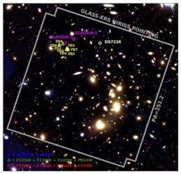
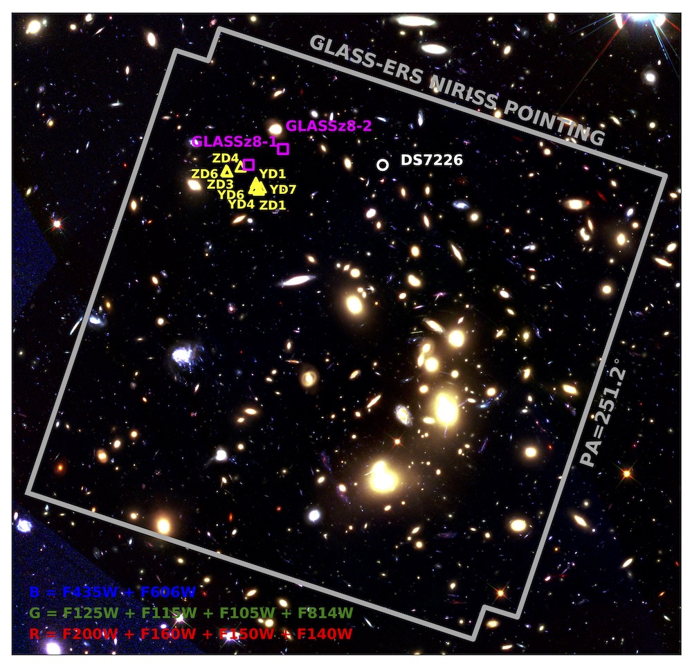
This representative-color image combines new observations with JWST and previous observations with the Hubble Space Telescope. The two high-redshift galaxies confirmed in this work are marked with magenta squares. [Roberts-Borsani et al. 2022]

In the first of the five articles published today, a team led by Guido Roberts-Borsani (University of California, Los Angeles) carried out the first search for continuum emission from galaxies behind Abell 2744 with redshift z ≥ 7, corresponding to less than about 800 million years after the Big Bang.

Many searches for high-redshift galaxies rely on identifying prominent emission lines, but these spectral features are weakened from absorption by the neutral hydrogen gas present early in the epoch of reionization. As a result, high-redshift galaxies identified through spectral features in this time period are biased toward those with exceptionally bright emission lines. In order to identify galaxies more typical of this epoch, Roberts-Borsani and collaborators searched for continuum emission from highly lensed galaxies using 15 hours of NIRISS observations. Ultimately, the team confirmed the detection of two galaxies from that epoch with redshifts z = 8.04 and z = 7.90. The team also made tentative identifications of ultraviolet emission lines redshifted into JWST’s observing range, the presence of which may indicate low-metallicity star-forming regions or non-thermal photon sources.

image of Abell 2744

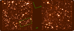
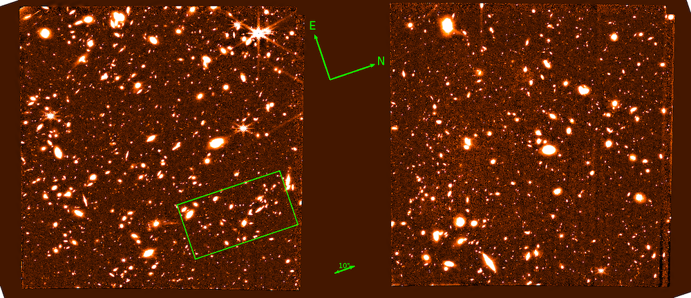
Reduced image of the field (split into module b, left, and module a, right) in the F444W filter, the reddest of the NIRCam wide-band filters. [Adapted from Merlin et al. 2022]

Image Reduction and Catalog Production

Emiliano Merlin (Italy’s National Institute for Astrophysics — Astronomical Observatory of Rome) and collaborators described their efforts to process and make available the NIRCam observations of Abell 2744. The observations, which are centered on the galaxy cluster, consist of images taken in seven filters from 0.9 to 4.4 microns.

In preparation for their planned photometric analysis, the team generated synthetic images from mock galaxy catalogs and used these images to test their image reduction pipeline, which is a customized version of the official JWST pipeline provided by the Space Telescope Science Institute. Ultimately, the team extracted 6,368 sources from the images and measured colors and fluxes for each source, all of which have been made publicly available along with the processed images.

Distant Galaxy Candidates

plot of the photometric measurements for one of the high-redshift galaxy candidates

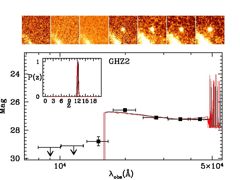
Photometry and best-fitting spectral energy distribution for the galaxy candidate at z = 12.2. The images across the top of the plot show the source in the seven wide-band NIRCam filters. [Adapted from Castellano et al. 2022]

Marco Castellano (Italy’s National Institute for Astrophysics — Astronomical Observatory of Rome) and coauthors pushed the search for early galaxies to extremely high redshifts. The team used two methods to identify potential galaxies with redshift z ~ 9–15 — just a few hundred million years after the Big Bang. The first method relies on a synthetic galaxy catalog — using observations of low- and moderate-redshift galaxies to predict the characteristics of high-redshift galaxies — to estimate the colors of galaxies in the desired redshift range. The second method uses photometric redshift, which relies on the overall reddening of a galaxy’s emission with increasing distance.

In total, the team identified six potential galaxies with redshifts in the z ~ 9–15 range. Two sources with redshifts of z = 10.6 and z = 12.2 were found to be especially intrinsically bright, with high rates of star formation. The remaining candidates, which were placed at slightly lower redshifts, were identified less robustly, and the authors note that spectroscopic followup and further deep imaging is needed to make a final identification.

From Reionization to Cosmic Noon

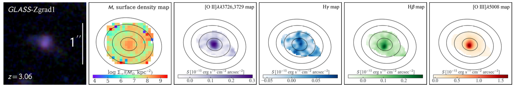
The penultimate article of those released today explores a galaxy somewhat less remote, situated in the star-formation heyday of z ≅ 1–3. A team led by Xin Wang (University of the Chinese Academy of Sciences; Chinese Academy of Sciences; California Institute of Technology) used JWST’s high-resolution spectroscopic capabilities to investigate a redshift z = 3.06 galaxy in detail, mapping the properties of its gas as a function of location within the galaxy.

This set of observations — the first instance of using JWST’s slitless spectroscopy to obtain spatially resolved observations of a high-redshift galaxy — allowed the team to measure the galaxy’s star-formation rate, metallicity, and extinction. The team found that the galaxy’s metallicity gradient is inverted, meaning that the galaxy’s outskirts contain more metals than the galactic center. This suggests that a past interaction between the target galaxy and a nearby galaxy that’s 100 times more massive caused metal-poor gas from the galaxy’s outer regions to be funneled in toward the center.

maps of stellar surface density and several emission lines within the galaxy GLASS-Zgrad1

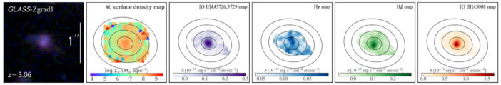
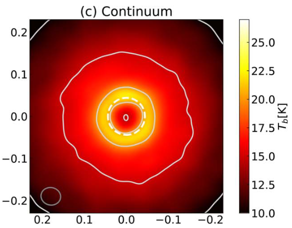
Maps of the galaxy GLASS-Zgrad1 constructed from JWST NIRISS observations. [Adapted from Wang et al. 2022]

A Visual-Wavelength View of Galaxy Sizes

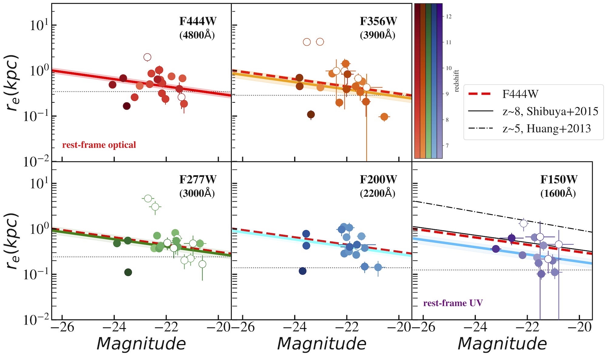
Finally, Lilan Yang (University of Tokyo) and collaborators investigated the size–luminosity relation for galaxies with redshift z > 7. While the Hubble Space Telescope has allowed researchers to measure the sizes of distant galaxies at rest-frame ultraviolet wavelengths, the size–luminosity relationship at rest-frame optical wavelengths has been more difficult to determine.

plots of the size–luminosity relationship for galaxies in the early universe.

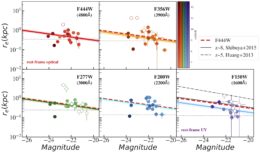
Size–luminosity relationships for galaxies observed in five NIRCam wavelength bands. The solid and dot-dashed black lines in the rightmost panel (F150W) show the results from previous studies with Hubble data. Click to enlarge. [Yang et al. 2022]

Using NIRCam, Yang and coauthors measured the sizes of 19 bright galaxies with redshifts 7 < z < 15. The team found that the slope of the size–luminosity relationship is somewhat steeper in the shortest wavelength band, caused by the faintest galaxies in their sample appearing comparatively small in that wavelength range. This may support previous findings based on Hubble observations that the size–luminosity relationship is best represented by a broken power law, with the faintest galaxies behaving differently from the brightest galaxies. However, the authors caution that this work is preliminary, and further analysis on a more complete sample of galaxies should provide greater clarity.

While the first five articles in the focus issue stick close to the stated goals of the GLASS-JWST program, the remaining articles will branch out to explore a wide range of topics — proto-globular clusters in Abell 2744, galaxy shapes during the epoch of reionization, intriguing foreground stars in the Abell 2744 field, and much more. Whet your appetite for early-release science with today’s research articles, and stay tuned for more results from GLASS-JWST!

Citation

“Early Results from GLASS-JWST. I: Confirmation of Lensed z ≥ 7 Lyman-break Galaxies behind the Abell 2744 Cluster with NIRISS,” Guido Roberts-Borsani et al 2022 ApJL 938 L13. doi:10.3847/2041-8213/ac8e6e

“Early Results from GLASS-JWST. II. NIRCam Extragalactic Imaging and Photometric Catalog,” Emiliano Merlin et al 2022 ApJL 938 L14. doi:10.3847/2041-8213/ac8f93

“Early Results from GLASS-JWST. III. Galaxy Candidates at z ∼9–15,” Marco Castellano et al 2022 ApJL 938 L15. doi:10.3847/2041-8213/ac94d0

“Early Results from GLASS-JWST. IV. Spatially Resolved Metallicity in a Low-mass z ∼ 3 Galaxy with NIRISS,” Xin Wang et al 2022 ApJL 938 L16. doi:10.3847/2041-8213/ac959e

“Early Results from GLASS-JWST. V: The First Rest-frame Optical Size–Luminosity Relation of Galaxies at z > 7,” L. Yang et al 2022 ApJL 938 L17. doi:10.3847/2041-8213/ac8803

A photograph of an astronaut on the lunar surface standing over an instrument with large solar panels

In the half-century since astronauts walked on the Moon, many of the practices and techniques used by earth-bound planetary scientists have evolved. Recently, a team of planetary scientists reprocessed Apollo-era seismic data to meet modern forms, ensuring that these precious measurements remain usable for the next generation.

Far-Flung Seismographs

The Apollo astronauts left more than footprints when they departed the Moon over fifty years ago. A few of these remnants were abandoned intentionally to continue the scientific mission in the years following each lunar departure: these were the passive seismometers, or devices designed to measure tiny displacements of the ground caused by seismic waves traveling through the Moon’s interior.

Despite the remoteness of their locale and its penchant for destroying complex technology, these instruments performed spectacularly. While they sat patiently listening, each of the five packages recorded numerous lunar quakes and meteor impacts, which collectively demonstrated that the lunar subsurface was a highly fractured, messy arrangement of rock.

A plot showing the vertical displacement of the ground as a function of time following a shallow moonquake. The displacement oscillates around zeros, and its amplitude decays with time.

The seismic profile of a representative shallow moonquake. The y-axis denotes vertical ground displacement in nanometers. This event was recorded by the package deployed at the Apollo 12 landing site. [Adapted from Nunn et al. 2022]

Initial Transmission

The success of these seismometers was hard fought, however, and depended just as much on the ground logistics as it did on the space hardware. The relatively simple instruments could not store data, and instead screamed their findings in real time across the void towards Earth. These shrieks, manifested as radio transmissions, were picked up by NASA’s Deep Space Network and recorded on magnetic reels, which later were copied to cassette tapes and eventually digitized.

This process offered numerous opportunities for errors. For one, the pace of the seismometer’s measurements was not steady, making timestamping each discrete sample difficult. For another, certain sections were missing or duplicated, depending on the number of Deep Space Network dishes able to receive broadcasts. Finally, small sections of data were corrupted each time a magnetic tape was copied over the intervening decades.

As a result, the previously digitized version of the seismometer data was full of holes, repeats, and uneven timestamps. Though it could be used, it could not be imported into modern seismic data processing software and required intimate knowledge of mission specifics not familiar to most practicing planetary scientists.

A two panel plot showing a seismogram before and after cleaning. The "before" version contains several spikes greater than 20x the amplitude of the signal. These spikes are missing in the "after" version.

Top: A portion of the seismic data prior to any cleaning. Bottom: The same portion after application of the authors’ cleaning and timestamp alignment procedures. [Nunn et al. 2022]

Cleaning and Archiving

In this new study, Ceri Nunn (NASA JPL) and collaborators undertook the Herculean task of extracting the data from the magnetic tapes, massaging them into a modern format, and archiving it digitally for future use. The team states that they “hope that the new archive will make it easier for a new generation of seismologists to use these data to learn more about the structure of the Moon,” and thanks to their efforts, that new generation can lean on the efforts of their predecessors.

The newly archived data can be found here.

Citation

“A New Archive of Apollo’s Lunar Seismic Data,” Ceri Nunn et al 2022 Planet. Sci. J. 3 219. doi:10.3847/PSJ/ac87af

1 31 32 33 34 35 112