Features RSS

A graphic of a white star surrounded by a pink haze of radiation. Streams of white particles flow away from the surface in lines, presumably following the magnetic field lines.

They’re powerful, they’re fast, and we aren’t sure about what causes them, but astronomers are closer than ever to understanding the source of mysterious fast radio bursts.

Flashes Without a Cause

Fast radio bursts: one of the most recent mysteries to appear in the sky and one of the most active fields of astronomical research. Since the discovery of the first of these powerful <1-second eruptions eruptions of radio waves back in 2007, astronomers have recorded hundreds of similar events. We know that they must originate from beyond our Milky Way galaxy, but, beyond that, astronomers have still yet to settle on a consensus about what might cause such brief, energetic flashes. This mystery of the origins of these bursts has driven many astronomers into an exciting, frustrating, and increasingly productive quest to understand whatever immense forces power them.

It is not easy to study a flash; by their very nature, they appear for only a fraction of a second, then vanish to almost never return. While a precious few do eventually repeat, they do so at largely irregular intervals, meaning astronomers can never really be sure when or where a fast radio burst might happen. The ones astronomers do manage to spot are almost always flagged by survey telescopes that scan huge swaths of the sky at once. A wide field of view comes with a tradeoff, though: although these telescopes can monitor enough sky that they have a good chance of catching a burst, their view of the sky is fairly blurry. So, although astronomers have recorded a few hundred bursts by now, they usually can’t say exactly where each one came from.

For the 16 years since the discovery of the first fast radio burst, astronomers have been trying to piece together their secrets without even knowing the location of each flash. Recently, however, they have made progress both in narrowing in on their quarry and on understanding their source. Below are three recent studies published in AAS Journals detailing this progress.

A pixelated image of a galaxy that appears as a roughly circular blob at center. The white circle marking the uncertainty in the position of the FRB is much smaller than the galaxy itself.

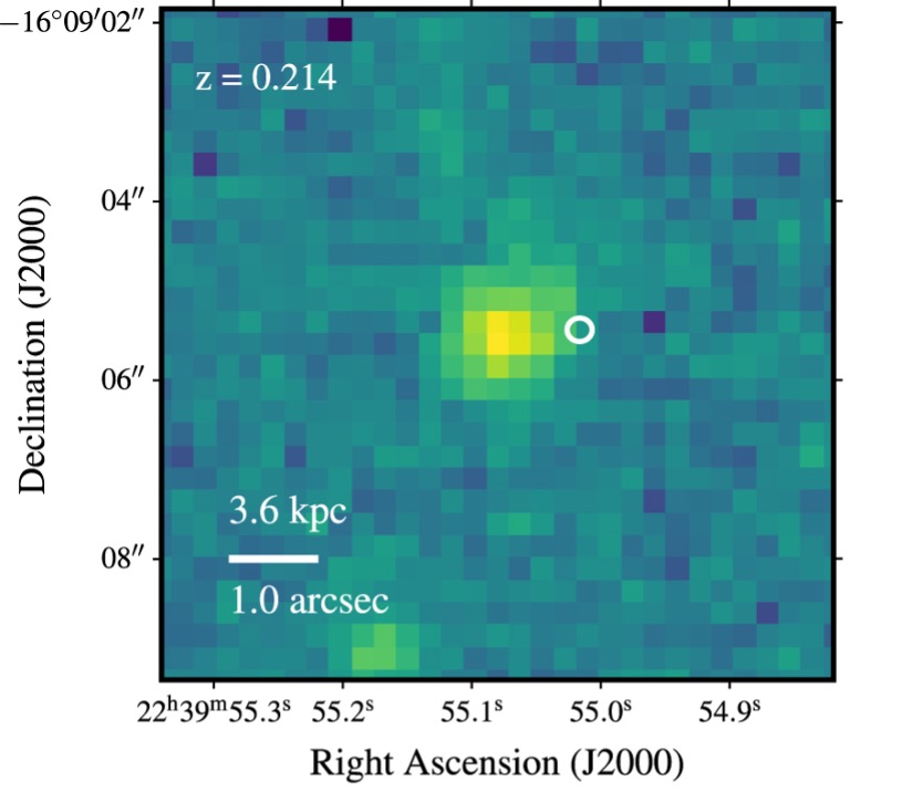
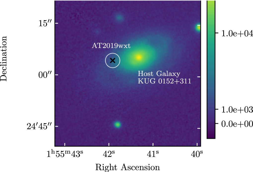
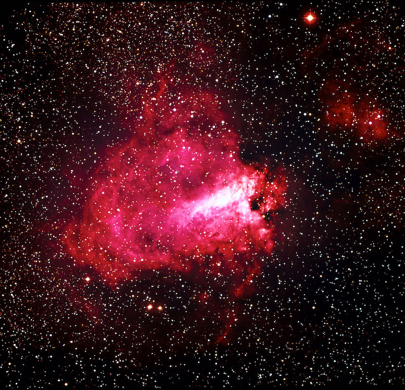
The location of the fast radio burst (white circle) and an image of the host galaxy. This galaxy sits at a redshift of z = 0.214. [Adapted from Bhandari et al. 2023]

First up is a study published in May of this year by a team led by Shivani Bhandari, Netherlands Institute for Radio Astronomy. Bhandari and collaborators describe their discovery of a fast radio burst using the Australian Square Kilometre Array Pathfinder, a relatively new and phenomenally capable radio telescope that they used the pin down the location of the flash to within one arcsecond (about 0.03% of a degree!). This extreme precision allowed the team to identify which galaxy the flash came from, and what they found was somewhat surprising: the host was a small, somewhat boring dwarf galaxy with almost no ongoing star formation. This is in contrast to the handful of known hosts of repeating fast radio burst, which were all more lively, active galaxies. Considering both the host and the properties of the burst itself, the team concluded that their burst could have been caused by an “accretion jet from a hyperaccreting black hole.”

Magnetar Earthquakes?

A month later in early June, a team led by Fayin Wang, Nanjing University, published their own analysis of archival data to suggest an alternative source. By digging through all of the observations of two known repeating fast radio burst collected by the Five-hundred-meter Aperture Spherical radio Telescope (FAST), Wang and colleagues realized that the gaps between bursts were not quite as random as previously thought. Instead, whatever was causing the bursts seemed to have “memory,” meaning the triggers must be correlated in time. Building from this, they advocate for a different explanation, positing that the bursts occur whenever a highly magnetized neutron star undergoes “crustal fractures” — in other words, earthquakes. After a shift, the magnetic stresses will build up again and cause the process to repeat, which could give rise to the recurring bursts.

More Than One

A photograph of two nearby spiral galaxies, with cyan ellipses overplotted to show the uncertainty in the location of the FRB.

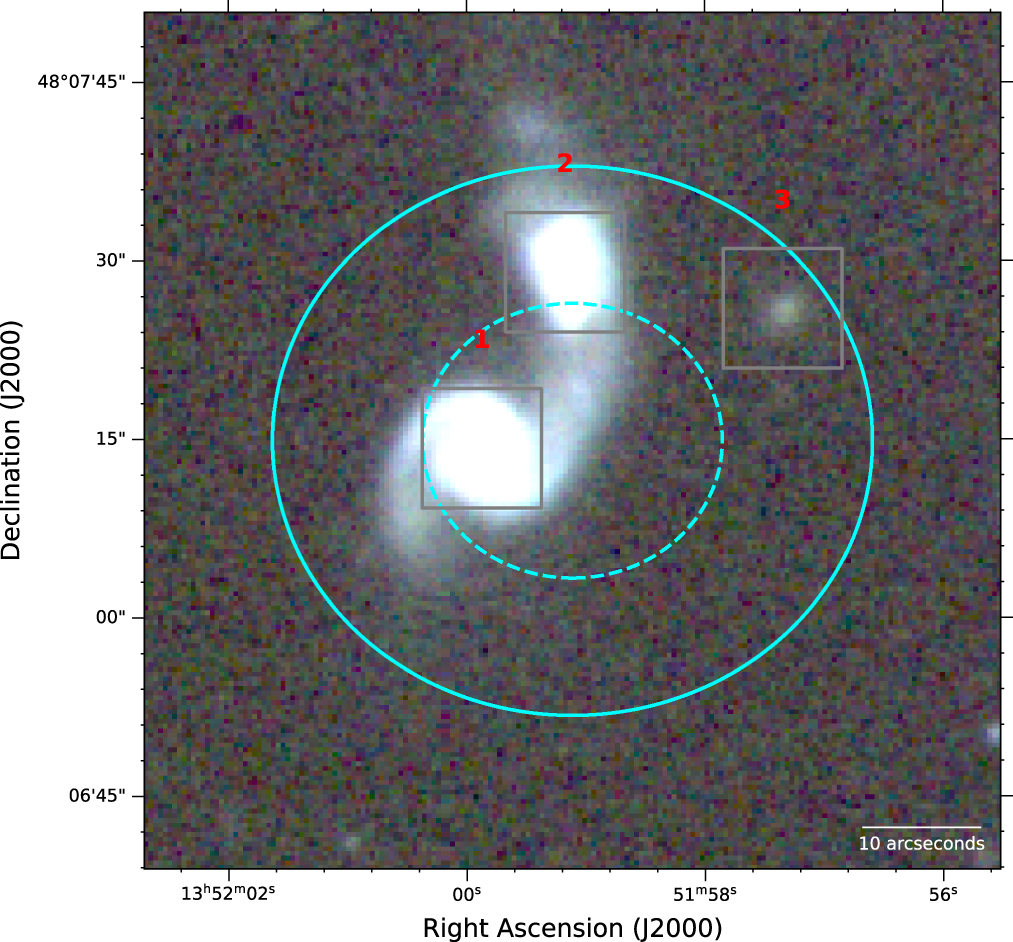
The location of one of the thirteen repeating fast radio burst, which lines up perfectly with a pair of merging spiral galaxies. [Michilli et al. 2023]

Finally, in late June, another study led by Daniele Michilli, Massachusetts Institute of Technology, offered a bridge between the two previous ones. This publication describes a re-analysis of data collected by the Canadian Hydrogen Intensity Mapping Experiment (CHIME), which resulted in newer, much more precise estimates of previous fast radio burst locations. The team focused on 13 repeating bursts and pinned down each of their locations to within about 10 arcseconds. While that isn’t precise enough to nail the host galaxy for all 13, they did mange to conclusively identify the host for two of them. Intriguingly, these two galaxies were nothing alike: one is a peaceful, quiescent galaxy, and the other is one in a pair of merging spiral galaxies that are actively forming many stars. This suggests that fast radio burst can come from a range of environments, or even that there could be multiple causes that each produce a similar looking signal.

While the final, well-supported model to describe all fast radio burst is still out of reach, astronomers are actively getting closer to this final goal. As new telescopes and processing techniques come online, it is only a matter of time until enough data is collected and analyzed that a clearer picture emerges. Soon, what now appear as mysterious flashes will be the subjects of well-documented chapters in the next textbooks, and this knowledge will be based on studies happening today, like these three.

Citation

“A Nonrepeating Fast Radio Burst in a Dwarf Host Galaxy,” Shivani Bhandari et al 2023 ApJ 948 67. doi:10.3847/1538-4357/acc178

“Repeating Fast Radio Bursts Reveal Memory from Minutes to an Hour,” F. Y. Wang et al 2023 ApJL 949 L33. doi:10.3847/2041-8213/acd5d2

“Subarcminute Localization of 13 Repeating Fast Radio Bursts Detected by CHIME/FRB,” Daniele Michilli et al 2023 ApJ 950 134. doi:10.3847/1538-4357/accf89

illustration of a quasar

Using JWST, researchers have validated a new tool for studying quasars — the extremely luminous nuclei of galaxies in the early universe, powered by the accretion of gas onto a growing supermassive black hole.

Studying Superlative Sources

Hubble image of the quasar 3C 273

This Hubble image shows the quasar 3C 273. [ESA/Hubble & NASA; CC BY 4.0]

Quasars are among the most luminous objects in the universe. Not only are they extremely bright, some quasars also create immense outflows that inject even more energy into their surroundings. The energy generated by quasars is enough to turn the tides of star formation in entire galaxies, transforming busy, star-forming galaxies into quiescent ones.

Astronomers have identified the best optical wavelengths for studying quasar outflows, but with a powerful new infrared telescope in our toolkit, we’ll need to develop new diagnostics for studying these features in the infrared and measure how they stack up against our existing tools.

Visible vs. Infrared

To expand our toolkit into the infrared, David Rupke (Rhodes College) and collaborators compared infrared observations from JWST and visible-light observations from the Gemini North telescope. The team focused on the quasar F2M110648.35+480712.3, or F2M1106 for short, which at roughly 5 billion light-years away is the nearest of the quasars in the JWST Q3D Early Release Science program sample.

Rupke‘s team analyzed observations at two main wavelengths: visible light at 500 nanometers, which comes from oxygen atoms that have lost two of their electrons, and infrared light at 10.5 microns (1 micron = 10-6 meter), which comes from sulfur atoms that have lost three of their electrons. The 500-nanometer oxygen line is a proven tool for studying quasar outflows since it traces oxygen atoms that have lost their electrons to the harsh ultraviolet radiation from the quasar. Coincidentally, it takes nearly the same amount of energy to remove three electrons from a sulfur atom as it does to steal two electrons from an oxygen atom. This hints that the infrared sulfur line might trace the same structures that are traced by the oxygen line — namely, the warm, ionized gas that makes up a quasar’s powerful outflows.

Future Quasar Investigations

comparison of emission from oxygen and sulfur atoms in the outflow region of a quasar

Comparison of emission from doubly ionized oxygen (OIII) at 500 nm/5007 Å to emission from triply ionized sulfur (SIV) at 10.51 microns. Click to enlarge. [Rupke et al. 2023]

Imaged at 500 nanometers, the quasar F2M1106 clearly has two lobes extending roughly 33,000 light-years out from the quasar in opposite directions. At 10.5 microns, the scene is similar, with two oppositely directed lobes with their brightest points located at the same position at both wavelengths.

While the two emission lines don’t paint exactly the same picture — the infrared sulfur line is inherently weaker than the optical oxygen line, so it fades out of view in certain regions — it’s clear that 10.5-micron emission is an effective way to study quasar outflows with JWST. And for dust-reddened quasars like F2M1106, it has a particular advantage, as its longer wavelength is better at piercing dusty clouds. This study demonstrates JWST’s potential as a new tool for studying quasar outflows, helping us to understand the impact of these structures on galaxy evolution.

Citation

“First Results from the JWST Early Release Science Program Q3D: Benchmark Comparison of Optical and Mid-infrared Tracers of a Dusty, Ionized Red Quasar Wind at z = 0.435,” David S. N. Rupke et al 2023 ApJL 953 L26. doi:10.3847/2041-8213/aced85

ultraviolet image of Mars

As the Sun’s magnetic activity cycle ramps up, solar storms are brewing. A recent research article describes what two Mars-orbiting spacecraft saw when a solar storm struck the red planet.

image of the Sun releasing two coronal mass ejections

This image from the Solar and Heliospheric Observatory shows two coronal mass ejections during an event in November 2000. [ESA/NASA/SOHO]

Storms from the Sun

The Sun’s atmosphere is suffused with pent-up magnetic energy that periodically escapes, powering coronal mass ejections (CMEs): immense eruptions of plasma and magnetic fields. CMEs are common — the frequency varies from about 50 a year when the Sun is at its calmest to more than 1,000 a year at the peak of the Sun’s activity cycle — but only a small fraction of these storms strike the planets in our solar system.

When a CME strikes Earth, it disturbs and compresses our planet’s protective magnetic shield and creates brilliant auroras. While Earth has a strong global magnetic field to shield our atmosphere from these storms, other planets are not as fortunate. Mars has feeble magnetic fields buried in some of its crust, perhaps a remnant of a stronger and larger magnetic field from long ago, but its atmosphere is largely unprotected. How solar activity like CMEs affects the atmosphere of Mars is important for our understanding of how the red planet’s atmosphere and habitability has evolved over billions of years.

Day and Night

On 4 December 2021, a CME burst from the Sun. Two days later, it swept past the BepiColombo spacecraft, which was surfing through the solar wind after passing close to Mercury for the first time, and charged toward Mars. There, two spacecraft stood at the ready: Tianwen-1 and MAVEN. When the CME reached Mars on 10 December 2021, Tianwen-1 witnessed the impact head on from its vantage point on the sunlit side of the planet. MAVEN took notes from the night side, spared the direct impact of the CME but positioned to witness how its effect propagated around the planet.

illustration of the orbits of Tianwen-1 and MAVEN during the CME

An illustration of the orbits of the Tianwen-1 and MAVEN spacecraft during the CME’s passage. Tianwen-1 sampled the day side atmosphere while MAVEN measured the night side atmosphere. BepiColombo witnessed the event from much closer to the Sun. Click to enlarge. [Yu et al. 2023]

A team led by Bingkun Yu (Institute of Deep Space Sciences) described the impact of the CME on Mars from the perspective of these two spacecraft. These spacecraft monitor Mars’s ionosphere, a weakly ionized layer of the atmosphere created by high-energy solar photons. As the CME reached Tianwen-1 on Mars’s day side, it compressed the ionosphere, pushing the top of this layer progressively lower over the course of several days.

Under normal conditions, some ionospheric plasma travels around the planet to its night side. What MAVEN witnessed as the CME raged on was notably different: a major decrease in the number of ions present in the shadow of the planet. This decrease suggests that rather than swinging around to the night side, the ions were escaping the atmosphere altogether, swept downstream by the CME.

Escape of Martian Plasma

plot summarizing the effects of the CME on the Martian ionosphere

Summary of the effects of the interplanetary CME (ICME) on Mars’s ionosphere. The density of the ionospheric plasma, shown by the solid lines, dipped, and the ionopause — the altitude above with the plasma density drops off sharply — was pushed lower day by day. Click to enlarge. [Adapted from Yu et al. 2023]

Essentially, Yu and collaborators reported that Tianwen-1 and MAVEN witnessed the removal of ions from Mars’s atmosphere by the CME. MAVEN saw a loss of 34%, 61% and 73% of the electrons, O+ ions, and O2+ ions, respectively, from altitudes above 180 km.

Since only a small fraction of Mars’s atmosphere is ionized, this means the CME stole just a tiny amount of the atmosphere — but the compounded effects of CMEs over billions of years could be huge; the theft of ions likely shaped the evolution of Mars’s atmosphere, playing a role in transforming our neighboring planet from one that was warm and hospitable to the unforgiving, arid world it is today.

Citation

“Tianwen-1 and MAVEN Observations of the Response of Mars to an Interplanetary Coronal Mass Ejection,” Bingkun Yu et al 2023 ApJ 953 105. doi:10.3847/1538-4357/acdcf8

A circular red gas bubble, more opaque on the edges than in the center, sits in a field of stars.

In astronomy, not detecting something can tell us something useful. A recent article details a radio search for six supernovae that resulted in no detections — but still gives us hints about the companions of these exploding stars.

How Stars Explode

Illustration of a white dwarf accreting gas from a red giant companion star

Accretion from a companion star onto a white dwarf is one way to trigger a supernova. [Still image from an animation by NASA’s Goddard Space Flight Center Conceptual Image Lab]

Supernovae happen in two main ways. In the first, a massive star loses its battle with gravity, and its outer layers rebound off its collapsed core in a massive explosion. In the second, an evolved low- to intermediate-mass star experiences pulsations that cause its outer layers to gently waft off into space, leaving behind its core as a white dwarf. If the white dwarf has a binary companion, the companion can donate material to the white dwarf through winds, accretion, or a collision. If the white dwarf gains too much mass, its core ignites and the star explodes.

Researchers suspect that nearly any type of star, from compact white dwarfs to puffed-up supergiants, can donate mass to a white dwarf and trigger a supernova. Which stars actually do is an active area of research, especially since these explosions are useful cosmic distance markers. But how can we tell from the aftermath of the explosion what kind of star was involved?

A Rapid Radio Search

When a star donates mass to its white dwarf companion, some of that gas remains in the space between the two stars, and the distribution of the gas can tell us about the type of companion star; for example, the billowing stellar winds of a supergiant should create an extended region of low-density gas. When a supernova’s shock wave collides with and compresses this gas, it generates synchrotron radiation from electrons traveling in helical paths around magnetic field lines. Synchrotron radiation is produced even when the supernova collides with very low-density material that would be impossible to see through other means.

Chelsea Harris (Michigan State University) and collaborators performed a search for synchrotron radiation from six nearby supernovae that had been detected at optical wavelengths. Judging by the evolution of their optical light curves, these supernovae all resulted from exploding white dwarfs with mass-donating stellar companions. However, the team found no radio emission to accompany the rapidly fading optical light of any of the supernovae in their sample.

Plot showing the types of winds ruled out by the radio non-detections of the supernovae in the authors' sample

Non-detections of the six supernovae rule out winds with the parameters spanned by the green bars. Click to enlarge. [Harris et al. 2023]

Winds, Shocks, and Shells

By modeling how much radio emission we’d expect to see from various distributions of circumstellar gas, the team was able to rule out the presence of low-density stellar winds from a supergiant companion. The non-detections also ruled out most winds due to accretion of material onto the white dwarf.

As part of their investigation, Harris and collaborators also modeled the expected synchrotron emission from a shock wave colliding with a dense shell of circumstellar gas. This scenario might arise when a pre-supernova white dwarf undergoes one or more novae before the ultimate explosion. Unexpectedly, the team found that these dense shells probably don’t produce a detectable amount of synchrotron emission. While radio observations are a powerful tool to study circumstellar gas, these shells might make themselves known on the other side of the electromagnetic spectrum, with fleeting bursts of X-rays or gamma rays.

Citation

“Radio Observations of Six Young Type Ia Supernovae,” C. E. Harris et al 2023 ApJ 952 24. doi:10.3847/1538-4357/acd84f

Andromeda Galaxy in ultraviolet

The cosmological constant, once rued by Einstein as his greatest blunder, is back in style. Researchers have used an entirely new method to determine the value of this constant — thought to be related to dark energy — using a galaxy in our cosmic backyard.

Accounting for Acceleration

image of the cosmic microwave background

An image of anisotropies in the cosmic microwave background. The Planck satellite studied the cosmic microwave background to measure several important cosmological parameters. [ESA and the Planck Collaboration]

Our universe is expanding, and that expansion is accelerating, propelled by a mysterious quantity known as dark energy. Many researchers suspect that dark energy is an explanation for the cosmological constant, a quantity tacked onto the equations of Einstein’s theory of gravity. Initially included as a way to make the equations describe a static, non-expanding universe, Einstein scrapped the constant when the universe was revealed to be expanding. With the discovery that this expansion is actually accelerating, the cosmological constant is back in vogue, but with a new purpose.

Researchers have devised a number of ways to measure quantities relevant to the cosmological constant. For example, the Planck mission mapped the tiny imperfections and non-uniformities in the cosmic microwave background — the oldest light in the universe — to measure the cosmological constant on a global scale. But as with all active areas of research, it’s important to make measurements in multiple ways to test our theories from all angles. How might we probe the cosmological constant on an entirely different scale?

an illustration of the local group of galaxies

An illustration of the Local Group of galaxies, which contains the Milky Way and Andromeda, as well as some of its near neighbors. Click to enlarge. [Antonio Ciccolella; CC BY 4.0]

Local Solutions to Global Questions

David Benisty, Anne-Christine Davis, and Wyn Evans (University of Cambridge) used pairs of galaxies locked in a gravitational dance to place constraints on the value of the cosmological constant. Their method hinges on the fact that the fabric of spacetime, from the space between the stars to the gaps between galaxies, is expanding under the influence of dark energy. This means that encoded within the orbital motions of any gravitationally bound galaxy pair is the subtle pressure of dark energy, forcing the galaxies apart as gravity pulls them together.

Benisty and collaborators analytically solved the two-body problem that describes the orbits of the Milky Way and its most massive neighbor, Andromeda, and accounts for the repulsive influence of dark energy. In doing so, they constrained the value of the cosmological constant over a few million light-years — a much smaller scale than the Planck mission, which drew its conclusions from the cosmic microwave background that suffuses the entire sky.

Upper Limits and Other Applications

plot of the constraints on the value of the cosmological constant placed by Planck and the method used in this work

Constraints on the cosmological constant, Λ, compared to the constraints determined from Planck data. Future measurements, such as with JWST, are anticipated to greatly improve the constraint placed by the binary galaxy method. [Adapted from Benisty et al. 2023]

The team’s findings agreed with the results from the Planck mission, finding an upper limit on the value of the cosmological constant equal to 5.44 times the value measured by Planck. While the constraint is not particularly stringent, Benisty and coauthors anticipate that more precise data will allow them to narrow the constraint in the future. In particular, stellar positions measured by JWST will improve our estimates of Andromeda’s mass, which is one of the largest sources of uncertainty.

Benisty and collaborators also used their method to place constraints on other theories of gravity. While these constraints were less restrictive than those placed on the cosmological constant, the technique is still valuable as it constrains modified gravity on scales of millions of light-years rather than the solar-system-sized scales from previous work.

Citation

“Constraining Dark Energy from the Local Group Dynamics,” David Benisty et al 2023 ApJL 953 L2. doi:10.3847/2041-8213/ace90b

A photograph of a masked-out star surrounded by a halo of light leaking around the edge of the mask. Surrounding the halo are smaller star-like dots, one of which is annotated with an arrow. This is the directly imaged planet, and the other dots are faint background stars.

Given JWST’s unprecedented capabilities, the first time it tries out a new instrument setting, it often sees something never before observed. Recently, that trend continued when JWST deployed its coronagraphic masks and snapped the first direct picture of an exoplanet in the mid-infrared.

New Settings

As has been noted repeatedly in AAS publications, JWST is a telescope like no other. For more than a year, scientists and the public alike have been spoiled with nearly weekly discoveries enabled by its unparalleled sensitivity. In exoplanet science especially, it has made good on its promise to revolutionize the field. Now, as JWST becomes a toddler and celebrates almost 20 months in space, astronomers are finishing up analyzing the last of its initial studies with each instrument and setting.

One of these studies, led by Aarynn L. Carter (University of California, Santa Cruz), describes JWST’s first attempts at high-resolution direct imaging of an exoplanet using its coronagraphic masks.

A Challenge, Even for the Best

Directly imaging an exoplanet is not an easy task: even planets that circle their host stars on wide, 100+ au orbits appear right next to them from our faraway vantage within the solar system. Additionally, planets are also much smaller, cooler, and therefore fainter than their hosts. Putting these two issues together, finding exoplanets by direct imaging is often compared to trying to see a firefly next to a floodlight from miles away.

Initial (leftmost column) and fully processed (right columns) images of HIP 65426b. Each row shows the planet through a different wavelength filter, and each column shows the result of a different processing technique. [Carter et al. 2023]

Luckily, JWST and other telescopes have a trick to deal with such domineering stars. A few of its instruments, including its Near Infrared Camera and Mid-Infrared Instrument, have tiny coronagraphic masks that can block most of a star’s light without shielding the area around it. Just as someone might block the Sun with their hand when trying to spot a plane flying overhead, by suppressing the parent star’s glare, JWST can see fainter nearby planets more clearly.

Even still, these masks cannot perfectly block out all of a star’s light, so image processing must be carried out back on the ground to cleanly extract any shy, small planets.

Impressive Performance 

So how did JWST do? Even better than its high expectations. Although its target, a super-Jupiter named HIP 65426b, is more than 1,000 times fainter than the very nearby parent star, JWST could easily disentangle the two in all seven filters the team observed through. Some of those filters only let through mid-infrared wavelengths of light, making this the first direct picture of an exoplanet taken beyond 5 microns (1 micron = 10-6 meter).

Three histograms describing the likelihood of the mass, effective temperature, and radius of HIP 65426b. The median values are 7.1 Jupiter masses, 1283 Kelvin, and 1.44 Jupiter radii, respectively.

Properties of HIP 65426b calculated by comparing JWST observations to evolutionary models. Click to enlarge. [Carter et al. 2023]

By comparing their observations to different models, the team measured the size and temperature of HIP 65426b more accurately than ever before. Possibly more exciting than their results about this specific planet, however, were the implications for studies to come. Since JWST barely broke a sweat finding this wide-orbiting super-Jupiter planet, Carter and collaborators estimate that under the right circumstances, JWST might be able to detect planets smaller than Saturn and within 10 au of their host star.

Planets this small and this close to their stars have never before been directly imaged. The fact that the next few years could include pictures of exoplanets similar to those in our solar system is a thrilling and surprising possibility, one brought about directly through the work that went into designing, building, and operating this miracle of a telescope.

Citation

“The JWST Early Release Science Program for Direct Observations of Exoplanetary Systems I: High-contrast Imaging of the Exoplanet HIP 65426 b from 2 to 16 μm,” Aarynn L. Carter et al 2023 ApJL 951 L20. doi:10.3847/2041-8213/acd93e

Hubble Space Telescope image of the massive star Eta Carinae

What started as the search for the source of a potential gravitational wave signal ended with the discovery of an unusual supernova. The supernova, SN2019wxt, showed a double-peaked light curve similar to previous ultra-stripped supernova candidates.

There and Gone

plot showing the location of the newly discovered transient

Location of the newly discovered transient, labeled AT2019wxt, in the outskirts of its host galaxy. [Shivkumar et al. 2023]

In December 2019, the LIGO and Virgo gravitational wave detectors distributed an alert for an event cataloged as S191213g, jump-starting a search for an electromagnetic counterpart to the possible gravitational wave signal. In the days following the alert, multiple telescopes turned toward the source region for the signal, homing in on a rapidly evolving object that was brightening the outskirts of a compact galaxy about half a billion light-years from Earth. Further analysis of S191213g downgraded its significance as a gravitational wave signal, ending the search for its source — but the newly discovered object got even more interesting.

“Just” a Supernova

In a recent research article, Hinna Shivkumar (University of Amsterdam) and collaborators outlined the follow-up observations of this intriguing target. As early data trickled in, the object remained hard to classify, though its mostly featureless spectrum with a broad emission line from helium marked it as an exploding star that had lost its outer layers of hydrogen, and it gained the label SN2019wxt.

optical and near-infrared light curve of the event

Optical and near-infrared light curves of SN2019wxt over three weeks following the initial detection. The i and g bands show the intriguing double-peaked shape. Click to enlarge. [SN2019wxt et al. 2023]

Shivkumar and coauthors used X-ray data from the Chandra X-ray Observatory, radio data from the Very Large Array, and optical images and spectra from telescopes across several continents to study the explosion further. Rather than showing a single peak to its light curve like a typical supernova, SN2019wxt peaked twice in just three days, making it one of the fastest-evolving supernovae known. Modeling of SN2019wxt’s light curve suggested that the first peak is due to rapid cooling of an expanding bubble of plasma, and the second peak is due to radioactive decay of material ejected in the explosion.

Double Peaked and Ultra-stripped?

Bolometric light curve compared to best-fitting models

Bolometric light curve of SN2019wxt (black circles) and best-fitting models of shock cooling (green dashed line) and radioactive decay (blue dashed line). [Shivkumar et al. 2023]

The unusual light curve, lack of hydrogen spectral lines, and modeled ejecta mass and explosion radius place SN2019wxt as a possible ultra-stripped-envelope core-collapse supernova. This rare class of supernovae contains only a few candidates, which are characterized by rapidly declining brightness, double-peaked light curves, and the presence of circumstellar material. These features point to stars that are stripped of much of their mass before exploding, leaving little material to be ejected in the explosion.

The serendipitous discovery of SN2019wxt makes for a great story, but to learn more about ultra-stripped supernovae in the future, we’ll need to catch them right when they happen. Luckily, the Vera C. Rubin Observatory’s long-awaited Legacy Survey of Space and Time draws ever closer, and after its anticipated start in 2025 will bring one million supernova detections each year — and thus millions of opportunities to study rare supernovae like SN2019wxt.

Citation

“SN2019wxt: An Ultrastripped Supernova Candidate Discovered in the Electromagnetic Follow-up of a Gravitational Wave Trigger,” Hinna Shivkumar et al 2023 ApJ 952 86. doi:10.3847/1538-4357/acd5d5

Hubble image of the galaxy NGC 4485

Do galaxies form stars steadily or in sudden bursts? In a new article, researchers study starlight from hundreds of galaxies to disentangle their star formation histories.

In the Light of New Stars

As new stars form, they heat and disrupt their surroundings. This process of feedback, which also includes things like supernovae and jets from accreting supermassive black holes, can moderate the rate at which a galaxy forms new stars. As a result, star formation sometimes happens in fits and starts. But how can we tell if a galaxy has experienced smooth or sudden star formation?

Omega Nebula or Messier 17

Messier 17, the Omega Nebula, glows red because of energy injected by hot young stars. [ESO; CC BY 4.0]

When we observe a galaxy, we see the combined light of billions of stars. By studying certain wavelengths of light, we can track the timeline over which some of that galaxy’s stars formed. Specifically, ultra-hot O and B stars ionize bubbles of hydrogen gas around them, causing the gas to glow red. This red H-alpha emission wanes just 5 million years after the onset of star formation, so detecting H-alpha emission from a galaxy clues us into recent star formation. Slightly cooler B stars and A stars, on the other hand, emit ultraviolet light steadily for about 200 million years. By measuring a galaxy’s ultraviolet and H-alpha light, we can study the galaxy’s star formation over the past 200 million years.

plots of ultraviolet-to-H-alpha ratio

Model output showing how the ultraviolet-to-H-alpha ratio, ζ, changes over time for constant star formation (red lines) and bursts of different durations (purple, blue, green, and cyan lines). Click to enlarge. [Adapted from Mehta et al. 2023]

Studying Star Formation History

Vihang Mehta (IPAC-Caltech) and collaborators determined the recent star formation histories for 979 galaxies using ultraviolet images and infrared spectra from the Hubble Space Telescope. These data sets allowed them to determine the ultraviolet emission from cooler B and A stars and the H-alpha emission from ionized gas surrounding hot O and B stars. (The galaxies in the sample are at redshifts between 0.7 and 1.5, so their red H-alpha emission has shifted into the infrared.)

Using these data, Mehta’s team calculated the ratio of ultraviolet to H-alpha emission for each galaxy. To interpret the results, the team modeled how steady and “bursty” star formation impact the ratio. In the case of steady star formation, the ratio increases slowly to a constant value. For a burst of star formation, the ratio jumps to high values before decreasing to a constant value.

Smooth vs. Bursty

Plot of the measured ultraviolet-to-H-alpha ratio

Measured ultraviolet-to-H-alpha ratio, corrected for dust attenuation, as a function of distance from the galactic center for galaxies in three mass bins. Low- and intermediate-mass galaxies do not have a strong trend with radius. Click to enlarge. [Mehta et al. 2023]

By stacking the galaxy images and averaging them azimuthally, the team tracked the relative importance of steady and bursty star formation as a function of distance from the galactic center.

Bursty star formation appears to be more important in the outskirts of these galaxies than at their centers. Breaking the galaxies into groups by mass, the team found that low- and intermediate-mass galaxies have bursty star formation throughout. High-mass galaxies, on the other hand, appear to have smooth star formation at their centers and bursty star formation at their edges. Looking at localized trends, the team also found that regions where stars are relatively sparse tend to have bursty star formation, regardless of the total mass of the galaxy.

The trends unearthed in this study will help to constrain our models of star formation. And as always, JWST data can help push this investigation to higher redshifts, even as far back as cosmic noon — when our universe’s star formation was at its peak.

Citation

“A Spatially Resolved Analysis of Star Formation Burstiness by Comparing UV and Hα in Galaxies at z ∼ 1 with UVCANDELS,” Vihang Mehta et al 2023 ApJ 952 133. doi:10.3847/1538-4357/acd9cf

illustration of the fully convective interior of a low-mass M-dwarf star

Researchers investigated the properties of M-dwarf stars within a gap discovered using Gaia spacecraft data to probe the connection between stellar structure and stellar activity.

Peering into the Interiors of Stars

plot of absolute magnitude versus color for low-mass stars

Absolute magnitude versus color, derived from Gaia spacecraft observations, for low-mass stars within 326 light-years of the Sun. A narrow gap appears where the density of data points is lower. [Jao et al. 2018]

Deep in the Sun’s interior, oceans of photons carry energy outward from the core. In the Sun’s outer layers, huge parcels of gas turn over and over, transporting energy to the surface through convection. This structure, consisting of a radiative interior and a convective exterior, is typical for stars like the Sun, but somewhere in the ranks of M dwarfs — the smallest, coolest, and most common type of star — the structure changes. The smallest M-dwarf stars are fully convective, their interiors churning all the way from their cores to their surfaces.

Surprisingly, we may actually be able to see the division between partially and fully convective stars! When plotting the absolute magnitudes and colors of thousands of stars — i.e., creating a Hertzsprung–Russell or H–R diagram — a narrow gap appears where relatively few stars exist. Research suggests that the stars in this gap have complex, unstable interiors and experience pulsations. The instability in these stars may drive large-scale changes to their magnetic fields, which may in turn manifest as stellar activity like starspots and stellar flares.

Plot showing active and inactive stars above, within, and below the gap

Left: Active and inactive stars in the eight subdivisions within the survey region (white dashed line). The background image has been enhanced to show the location of the gap (region E). Right: Same information, but also showing the equivalent width of the H-alpha line for the active stars. The equivalent width is a measure of the strength of the emission. Note that the two active stars below the gap edge (black line) have tiny equivalent widths. Click to enlarge. [Adapted from Jao et al. 2023]

A Deep Dive into the Gap

A team led by Wei-Chun Jao (饒惟君) from Georgia State University sought to understand how changing internal structure affects stellar activity. The team analyzed spectra of 480 nearby stars within the gap for signs of H-alpha emission, which is correlated with stellar activity. The distribution of stars with and without activity was remarkable: essentially all stars within the gap were inactive, with no H-alpha emission, and nearly all active stars fell above the gap.

To dive deeper into this finding, Jao and collaborators subdivided the stars in their sample into eight groups, four above the gap and four within and below the gap. On average, 15% of the stars above the gap are active, while just 1% of the stars within and below the gap are. This sharp division between active and inactive stars suggests that even though stars in the gap have a variety of internal structures, these variations don’t result in changing stellar activity as theorized.

Another Feature on the H–R Diagram

H–R diagrams showing the location of a newly identified activity gap

Left: Location of the second density dip and newly identified activity dip (yellow ellipse) relative to the gap and the study region from this work (white dashed region). Right: Percentage of stars showing activity. There is a dip in activity at the location of the yellow ellipse. Click to enlarge. [Adapted from Jao et al. 2023]

Jao and collaborators discovered something interesting about a different region of parameter space as well. There is another small section of the H–R diagram that is known to contain relatively few stars, and Jao’s team found that the stars in this region are less likely to be active than stars nearby. Since these stars lie just below the gap, they are the most massive stars that have fully convective interiors.

Why are stars in this region less active than their neighbors on the H–R diagram? It might be related to stellar rotation, since the stars in the activity dip are less likely to rotate rapidly than stars in surrounding areas on the diagram. This suggests that the most massive fully convective stars quickly spin down to slower speeds, possibly due to stellar winds that carry away angular momentum. Slower rotation means less pent-up magnetic energy and therefore less stellar activity. To investigate this theory further and gain a better understanding of the various gaps and dips on the H–R diagram, we’ll need more measurements of rotation rates and H-alpha emission for fully convective M dwarfs.

Citation

“Mind the Gap. I. Hα Activity of M Dwarfs Near the Partially/Fully Convective Boundary and a New Hα Emission Deficiency Zone on the Main Sequence,” Wei-Chun Jao et al 2023 AJ 166 63. doi:10.3847/1538-3881/ace2bb

A photograph of a comet against a background of many stars. The bright core is near the bottom-right, and the tail extends towards the upper-left, growing increasingly wispy and wide with distance to the core.

Where is all of the water around hyperactive comets coming from? A recent article asked if it could be “Ice, Ice, Maybe?” and concluded that it likely isn’t.

Icy Mystery

Comets spend most of their time far from the Sun, where it’s too cold (too cold) for ices trapped within their cores to sublime into gas. When their travels bring them inwards, though, these frozen materials transform into a gas cloud that escapes and enshrouds the nucleus. At this point, the comet is considered “active,” and though this happens to all comets, the severity of this outgassing varies widely. Some comets only sputter, and not much of their surfaces sublimes away. Others are mysteriously “hyperactive,” meaning they (go to the extreme) and produce so much water gas that it can’t all have come just from the surface layers of the nucleus.

One hypothesis claims that this excess water comes from ice grains near the surface of the nucleus. Though data collected in situ by robotic explorers confirm that these grains exist within at least some comets, these haven’t been observed on any aggressively outgassing objects and have not been conclusively linked to overabundant water.

The data and maximum likelihood model near-infrared spectrum of comet 46P. [Kareta et al. 2023]

To address this uncertainty, Theodore Kareta (Lowell Observatory) and a team of researchers (stopped, collaborated, and) observed a strange comet named 46P/Wirtanen in late 2018. Much like an early hip-hop artist, 46P was “hyperactive” in the 1990s and has steadily calmed down since. During its 1996–1997 close approach to the Sun, it threw off enough water that 100% of its surface must have been actively outgassing. By the time 46P came (back for a brand new) apparition in 2018, however, only 58% of its surface was contributing to gas production. Kareta and the team hoped to find icy grains near the core that could explain the earlier exuberance.

Ice-Free

A simulated image of 46P’s coma, oriented to match the viewing geometry of the real observations. [Kareta et al. 2023]

When reviewing their near-infrared reflectance spectrum, however, the team did not see the telltale absorption dips caused by water. Instead, the spectrum looked nearly featureless, with a red slope and nothing to indicate the presence of ice (vanilla or otherwise).

The team then went beyond a best-fit model and used a Markov chain Monte Carlo algorithm to put the tightest possible constraints on the amount of ice present. They found that, at most, water ice could make up <0.6% of 46P’s surface — not nearly enough to explain its previous hyperactivity.

Now the planetary science community is left with a problem: where is all of this water coming from? In principle, JWST could say “(yo I’ll solve it)” and turn its singularly capable suite of instruments on a few outgassing comets. Luckily, with plenty of fuel left and plenty of targets to choose from, we may get an answer in the next few years.

Citation

“Ice, Ice, Maybe? Investigating 46P/Wirtanen’s Inner Coma for Icy Grains,” Theodore Kareta et al 2023 Planet. Sci. J. 4 85. doi:10.3847/PSJ/accc28

“Ice Ice Baby,” Vanilla Ice 1990, Ichiban Records.

1 30 31 32 33 34 119