Features RSS

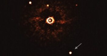
A photograph of a masked-out star surrounded by a halo of light leaking around the edge of the mask. Surrounding the halo are smaller star-like dots, one of which is annotated with an arrow. This is the directly imaged planet, and the other dots are faint background stars.

Given JWST’s unprecedented capabilities, the first time it tries out a new instrument setting, it often sees something never before observed. Recently, that trend continued when JWST deployed its coronagraphic masks and snapped the first direct picture of an exoplanet in the mid-infrared.

New Settings

As has been noted repeatedly in AAS publications, JWST is a telescope like no other. For more than a year, scientists and the public alike have been spoiled with nearly weekly discoveries enabled by its unparalleled sensitivity. In exoplanet science especially, it has made good on its promise to revolutionize the field. Now, as JWST becomes a toddler and celebrates almost 20 months in space, astronomers are finishing up analyzing the last of its initial studies with each instrument and setting.

One of these studies, led by Aarynn L. Carter (University of California, Santa Cruz), describes JWST’s first attempts at high-resolution direct imaging of an exoplanet using its coronagraphic masks.

A Challenge, Even for the Best

Directly imaging an exoplanet is not an easy task: even planets that circle their host stars on wide, 100+ au orbits appear right next to them from our faraway vantage within the solar system. Additionally, planets are also much smaller, cooler, and therefore fainter than their hosts. Putting these two issues together, finding exoplanets by direct imaging is often compared to trying to see a firefly next to a floodlight from miles away.

Initial (leftmost column) and fully processed (right columns) images of HIP 65426b. Each row shows the planet through a different wavelength filter, and each column shows the result of a different processing technique. [Carter et al. 2023]

Luckily, JWST and other telescopes have a trick to deal with such domineering stars. A few of its instruments, including its Near Infrared Camera and Mid-Infrared Instrument, have tiny coronagraphic masks that can block most of a star’s light without shielding the area around it. Just as someone might block the Sun with their hand when trying to spot a plane flying overhead, by suppressing the parent star’s glare, JWST can see fainter nearby planets more clearly.

Even still, these masks cannot perfectly block out all of a star’s light, so image processing must be carried out back on the ground to cleanly extract any shy, small planets.

Impressive Performance 

So how did JWST do? Even better than its high expectations. Although its target, a super-Jupiter named HIP 65426b, is more than 1,000 times fainter than the very nearby parent star, JWST could easily disentangle the two in all seven filters the team observed through. Some of those filters only let through mid-infrared wavelengths of light, making this the first direct picture of an exoplanet taken beyond 5 microns (1 micron = 10-6 meter).

Three histograms describing the likelihood of the mass, effective temperature, and radius of HIP 65426b. The median values are 7.1 Jupiter masses, 1283 Kelvin, and 1.44 Jupiter radii, respectively.

Properties of HIP 65426b calculated by comparing JWST observations to evolutionary models. Click to enlarge. [Carter et al. 2023]

By comparing their observations to different models, the team measured the size and temperature of HIP 65426b more accurately than ever before. Possibly more exciting than their results about this specific planet, however, were the implications for studies to come. Since JWST barely broke a sweat finding this wide-orbiting super-Jupiter planet, Carter and collaborators estimate that under the right circumstances, JWST might be able to detect planets smaller than Saturn and within 10 au of their host star.

Planets this small and this close to their stars have never before been directly imaged. The fact that the next few years could include pictures of exoplanets similar to those in our solar system is a thrilling and surprising possibility, one brought about directly through the work that went into designing, building, and operating this miracle of a telescope.

Citation

“The JWST Early Release Science Program for Direct Observations of Exoplanetary Systems I: High-contrast Imaging of the Exoplanet HIP 65426 b from 2 to 16 μm,” Aarynn L. Carter et al 2023 ApJL 951 L20. doi:10.3847/2041-8213/acd93e

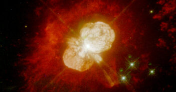
Hubble Space Telescope image of the massive star Eta Carinae

What started as the search for the source of a potential gravitational wave signal ended with the discovery of an unusual supernova. The supernova, SN2019wxt, showed a double-peaked light curve similar to previous ultra-stripped supernova candidates.

There and Gone

plot showing the location of the newly discovered transient

Location of the newly discovered transient, labeled AT2019wxt, in the outskirts of its host galaxy. [Shivkumar et al. 2023]

In December 2019, the LIGO and Virgo gravitational wave detectors distributed an alert for an event cataloged as S191213g, jump-starting a search for an electromagnetic counterpart to the possible gravitational wave signal. In the days following the alert, multiple telescopes turned toward the source region for the signal, homing in on a rapidly evolving object that was brightening the outskirts of a compact galaxy about half a billion light-years from Earth. Further analysis of S191213g downgraded its significance as a gravitational wave signal, ending the search for its source — but the newly discovered object got even more interesting.

“Just” a Supernova

In a recent research article, Hinna Shivkumar (University of Amsterdam) and collaborators outlined the follow-up observations of this intriguing target. As early data trickled in, the object remained hard to classify, though its mostly featureless spectrum with a broad emission line from helium marked it as an exploding star that had lost its outer layers of hydrogen, and it gained the label SN2019wxt.

optical and near-infrared light curve of the event

Optical and near-infrared light curves of SN2019wxt over three weeks following the initial detection. The i and g bands show the intriguing double-peaked shape. Click to enlarge. [SN2019wxt et al. 2023]

Shivkumar and coauthors used X-ray data from the Chandra X-ray Observatory, radio data from the Very Large Array, and optical images and spectra from telescopes across several continents to study the explosion further. Rather than showing a single peak to its light curve like a typical supernova, SN2019wxt peaked twice in just three days, making it one of the fastest-evolving supernovae known. Modeling of SN2019wxt’s light curve suggested that the first peak is due to rapid cooling of an expanding bubble of plasma, and the second peak is due to radioactive decay of material ejected in the explosion.

Double Peaked and Ultra-stripped?

Bolometric light curve compared to best-fitting models

Bolometric light curve of SN2019wxt (black circles) and best-fitting models of shock cooling (green dashed line) and radioactive decay (blue dashed line). [Shivkumar et al. 2023]

The unusual light curve, lack of hydrogen spectral lines, and modeled ejecta mass and explosion radius place SN2019wxt as a possible ultra-stripped-envelope core-collapse supernova. This rare class of supernovae contains only a few candidates, which are characterized by rapidly declining brightness, double-peaked light curves, and the presence of circumstellar material. These features point to stars that are stripped of much of their mass before exploding, leaving little material to be ejected in the explosion.

The serendipitous discovery of SN2019wxt makes for a great story, but to learn more about ultra-stripped supernovae in the future, we’ll need to catch them right when they happen. Luckily, the Vera C. Rubin Observatory’s long-awaited Legacy Survey of Space and Time draws ever closer, and after its anticipated start in 2025 will bring one million supernova detections each year — and thus millions of opportunities to study rare supernovae like SN2019wxt.

Citation

“SN2019wxt: An Ultrastripped Supernova Candidate Discovered in the Electromagnetic Follow-up of a Gravitational Wave Trigger,” Hinna Shivkumar et al 2023 ApJ 952 86. doi:10.3847/1538-4357/acd5d5

Hubble image of the galaxy NGC 4485

Do galaxies form stars steadily or in sudden bursts? In a new article, researchers study starlight from hundreds of galaxies to disentangle their star formation histories.

In the Light of New Stars

As new stars form, they heat and disrupt their surroundings. This process of feedback, which also includes things like supernovae and jets from accreting supermassive black holes, can moderate the rate at which a galaxy forms new stars. As a result, star formation sometimes happens in fits and starts. But how can we tell if a galaxy has experienced smooth or sudden star formation?

Omega Nebula or Messier 17

Messier 17, the Omega Nebula, glows red because of energy injected by hot young stars. [ESO; CC BY 4.0]

When we observe a galaxy, we see the combined light of billions of stars. By studying certain wavelengths of light, we can track the timeline over which some of that galaxy’s stars formed. Specifically, ultra-hot O and B stars ionize bubbles of hydrogen gas around them, causing the gas to glow red. This red H-alpha emission wanes just 5 million years after the onset of star formation, so detecting H-alpha emission from a galaxy clues us into recent star formation. Slightly cooler B stars and A stars, on the other hand, emit ultraviolet light steadily for about 200 million years. By measuring a galaxy’s ultraviolet and H-alpha light, we can study the galaxy’s star formation over the past 200 million years.

plots of ultraviolet-to-H-alpha ratio

Model output showing how the ultraviolet-to-H-alpha ratio, ζ, changes over time for constant star formation (red lines) and bursts of different durations (purple, blue, green, and cyan lines). Click to enlarge. [Adapted from Mehta et al. 2023]

Studying Star Formation History

Vihang Mehta (IPAC-Caltech) and collaborators determined the recent star formation histories for 979 galaxies using ultraviolet images and infrared spectra from the Hubble Space Telescope. These data sets allowed them to determine the ultraviolet emission from cooler B and A stars and the H-alpha emission from ionized gas surrounding hot O and B stars. (The galaxies in the sample are at redshifts between 0.7 and 1.5, so their red H-alpha emission has shifted into the infrared.)

Using these data, Mehta’s team calculated the ratio of ultraviolet to H-alpha emission for each galaxy. To interpret the results, the team modeled how steady and “bursty” star formation impact the ratio. In the case of steady star formation, the ratio increases slowly to a constant value. For a burst of star formation, the ratio jumps to high values before decreasing to a constant value.

Smooth vs. Bursty

Plot of the measured ultraviolet-to-H-alpha ratio

Measured ultraviolet-to-H-alpha ratio, corrected for dust attenuation, as a function of distance from the galactic center for galaxies in three mass bins. Low- and intermediate-mass galaxies do not have a strong trend with radius. Click to enlarge. [Mehta et al. 2023]

By stacking the galaxy images and averaging them azimuthally, the team tracked the relative importance of steady and bursty star formation as a function of distance from the galactic center.

Bursty star formation appears to be more important in the outskirts of these galaxies than at their centers. Breaking the galaxies into groups by mass, the team found that low- and intermediate-mass galaxies have bursty star formation throughout. High-mass galaxies, on the other hand, appear to have smooth star formation at their centers and bursty star formation at their edges. Looking at localized trends, the team also found that regions where stars are relatively sparse tend to have bursty star formation, regardless of the total mass of the galaxy.

The trends unearthed in this study will help to constrain our models of star formation. And as always, JWST data can help push this investigation to higher redshifts, even as far back as cosmic noon — when our universe’s star formation was at its peak.

Citation

“A Spatially Resolved Analysis of Star Formation Burstiness by Comparing UV and Hα in Galaxies at z ∼ 1 with UVCANDELS,” Vihang Mehta et al 2023 ApJ 952 133. doi:10.3847/1538-4357/acd9cf

illustration of the fully convective interior of a low-mass M-dwarf star

Researchers investigated the properties of M-dwarf stars within a gap discovered using Gaia spacecraft data to probe the connection between stellar structure and stellar activity.

Peering into the Interiors of Stars

plot of absolute magnitude versus color for low-mass stars

Absolute magnitude versus color, derived from Gaia spacecraft observations, for low-mass stars within 326 light-years of the Sun. A narrow gap appears where the density of data points is lower. [Jao et al. 2018]

Deep in the Sun’s interior, oceans of photons carry energy outward from the core. In the Sun’s outer layers, huge parcels of gas turn over and over, transporting energy to the surface through convection. This structure, consisting of a radiative interior and a convective exterior, is typical for stars like the Sun, but somewhere in the ranks of M dwarfs — the smallest, coolest, and most common type of star — the structure changes. The smallest M-dwarf stars are fully convective, their interiors churning all the way from their cores to their surfaces.

Surprisingly, we may actually be able to see the division between partially and fully convective stars! When plotting the absolute magnitudes and colors of thousands of stars — i.e., creating a Hertzsprung–Russell or H–R diagram — a narrow gap appears where relatively few stars exist. Research suggests that the stars in this gap have complex, unstable interiors and experience pulsations. The instability in these stars may drive large-scale changes to their magnetic fields, which may in turn manifest as stellar activity like starspots and stellar flares.

Plot showing active and inactive stars above, within, and below the gap

Left: Active and inactive stars in the eight subdivisions within the survey region (white dashed line). The background image has been enhanced to show the location of the gap (region E). Right: Same information, but also showing the equivalent width of the H-alpha line for the active stars. The equivalent width is a measure of the strength of the emission. Note that the two active stars below the gap edge (black line) have tiny equivalent widths. Click to enlarge. [Adapted from Jao et al. 2023]

A Deep Dive into the Gap

A team led by Wei-Chun Jao (饒惟君) from Georgia State University sought to understand how changing internal structure affects stellar activity. The team analyzed spectra of 480 nearby stars within the gap for signs of H-alpha emission, which is correlated with stellar activity. The distribution of stars with and without activity was remarkable: essentially all stars within the gap were inactive, with no H-alpha emission, and nearly all active stars fell above the gap.

To dive deeper into this finding, Jao and collaborators subdivided the stars in their sample into eight groups, four above the gap and four within and below the gap. On average, 15% of the stars above the gap are active, while just 1% of the stars within and below the gap are. This sharp division between active and inactive stars suggests that even though stars in the gap have a variety of internal structures, these variations don’t result in changing stellar activity as theorized.

Another Feature on the H–R Diagram

H–R diagrams showing the location of a newly identified activity gap

Left: Location of the second density dip and newly identified activity dip (yellow ellipse) relative to the gap and the study region from this work (white dashed region). Right: Percentage of stars showing activity. There is a dip in activity at the location of the yellow ellipse. Click to enlarge. [Adapted from Jao et al. 2023]

Jao and collaborators discovered something interesting about a different region of parameter space as well. There is another small section of the H–R diagram that is known to contain relatively few stars, and Jao’s team found that the stars in this region are less likely to be active than stars nearby. Since these stars lie just below the gap, they are the most massive stars that have fully convective interiors.

Why are stars in this region less active than their neighbors on the H–R diagram? It might be related to stellar rotation, since the stars in the activity dip are less likely to rotate rapidly than stars in surrounding areas on the diagram. This suggests that the most massive fully convective stars quickly spin down to slower speeds, possibly due to stellar winds that carry away angular momentum. Slower rotation means less pent-up magnetic energy and therefore less stellar activity. To investigate this theory further and gain a better understanding of the various gaps and dips on the H–R diagram, we’ll need more measurements of rotation rates and H-alpha emission for fully convective M dwarfs.

Citation

“Mind the Gap. I. Hα Activity of M Dwarfs Near the Partially/Fully Convective Boundary and a New Hα Emission Deficiency Zone on the Main Sequence,” Wei-Chun Jao et al 2023 AJ 166 63. doi:10.3847/1538-3881/ace2bb

A photograph of a comet against a background of many stars. The bright core is near the bottom-right, and the tail extends towards the upper-left, growing increasingly wispy and wide with distance to the core.

Where is all of the water around hyperactive comets coming from? A recent article asked if it could be “Ice, Ice, Maybe?” and concluded that it likely isn’t.

Icy Mystery

Comets spend most of their time far from the Sun, where it’s too cold (too cold) for ices trapped within their cores to sublime into gas. When their travels bring them inwards, though, these frozen materials transform into a gas cloud that escapes and enshrouds the nucleus. At this point, the comet is considered “active,” and though this happens to all comets, the severity of this outgassing varies widely. Some comets only sputter, and not much of their surfaces sublimes away. Others are mysteriously “hyperactive,” meaning they (go to the extreme) and produce so much water gas that it can’t all have come just from the surface layers of the nucleus.

One hypothesis claims that this excess water comes from ice grains near the surface of the nucleus. Though data collected in situ by robotic explorers confirm that these grains exist within at least some comets, these haven’t been observed on any aggressively outgassing objects and have not been conclusively linked to overabundant water.

The data and maximum likelihood model near-infrared spectrum of comet 46P. [Kareta et al. 2023]

To address this uncertainty, Theodore Kareta (Lowell Observatory) and a team of researchers (stopped, collaborated, and) observed a strange comet named 46P/Wirtanen in late 2018. Much like an early hip-hop artist, 46P was “hyperactive” in the 1990s and has steadily calmed down since. During its 1996–1997 close approach to the Sun, it threw off enough water that 100% of its surface must have been actively outgassing. By the time 46P came (back for a brand new) apparition in 2018, however, only 58% of its surface was contributing to gas production. Kareta and the team hoped to find icy grains near the core that could explain the earlier exuberance.

Ice-Free

A simulated image of 46P’s coma, oriented to match the viewing geometry of the real observations. [Kareta et al. 2023]

When reviewing their near-infrared reflectance spectrum, however, the team did not see the telltale absorption dips caused by water. Instead, the spectrum looked nearly featureless, with a red slope and nothing to indicate the presence of ice (vanilla or otherwise).

The team then went beyond a best-fit model and used a Markov chain Monte Carlo algorithm to put the tightest possible constraints on the amount of ice present. They found that, at most, water ice could make up <0.6% of 46P’s surface — not nearly enough to explain its previous hyperactivity.

Now the planetary science community is left with a problem: where is all of this water coming from? In principle, JWST could say “(yo I’ll solve it)” and turn its singularly capable suite of instruments on a few outgassing comets. Luckily, with plenty of fuel left and plenty of targets to choose from, we may get an answer in the next few years.

Citation

“Ice, Ice, Maybe? Investigating 46P/Wirtanen’s Inner Coma for Icy Grains,” Theodore Kareta et al 2023 Planet. Sci. J. 4 85. doi:10.3847/PSJ/accc28

“Ice Ice Baby,” Vanilla Ice 1990, Ichiban Records.

30 Doradus star-forming region

From its name alone, HD 222925 is no different from the 350,000 other stars in the Henry Draper Catalogue. What sets it apart is how closely we’ve studied it: we’ve measured the abundances of more elements in HD 222925 than any other star except for the Sun. This makes it an excellent target for studies of how stars inherit chemical elements from their birth environments.

Making Heavy Metals

Periodic table of elements showing the likely origin of each element

Periodic table of elements showing the likely origin of each element in our solar system. Click to enlarge. [Wikipedia user Cmglee; CC BY-SA 3.0]

The 65 elements identified in HD 222925’s spectrum include 42 elements heavier than iron. These heavy elements form when atoms capture neutrons, a process that can be either fast (multiple neutrons fusing onto an atom at once, before it can split apart into more stable atoms) or slow (single neutrons captured at a time). The rapid capture or r-process happens in extremely hot and dense environments like those created during supernovae, mergers of two neutron stars, or when a neutron star is ripped apart by a black hole.

Since stars form out of the gas left behind by previous generations of stars, the relative amounts of r-process elements in a star’s spectrum can tell us about the events that preceded it. In comparing HD 222925’s chemical abundance pattern to the Sun’s, researchers found that while the stars have similar heavy-metal abundance patterns overall, their patterns differ among the lighter r-process elements.

plot comparing the chemical abundance pattern of HD 222925 to that of the Sun

Comparison of HD 222925’s abundance pattern (black squares) to the Sun’s abundances due to slow neutron capture and rapid neutron capture, denoted s and r, respectively. Click to enlarge. [Holmbeck et al. 2023]

Going for the Gold (and Platinum and Iridium and…)

Researchers often model the Sun’s abundance pattern to test their understanding of how events like neutron star mergers create r-process elements. However, HD 222925 is older than the Sun and has a smaller amount of metals — elements heavier than helium — than the Sun does. This could mean that HD 222925’s chemical makeup reflects the r-process elements created in a single cataclysmic event, like two neutron stars colliding, rather than containing material enriched by multiple events. This would make HD 222925 a better template for the chemical abundance pattern created by a single source of r-process elements.

To address this possibility, Erika Holmbeck (Observatories of the Carnegie Institution for Science) and collaborators used computational models to determine the likeliest source — or sources — for the pattern of chemical elements seen in HD 222925.

More Adjustments Necessary

Holmbeck‘s team found that it was challenging to reproduce some of the star’s elemental abundances with models that included only one source of r-process elements, but they found two possible ways to bring the model into better agreement with the observations. In the first, HD 222925’s light and heavy r-process elements come from two different sources. In the second, there’s only one source — neutron star mergers — but conditions must be tuned in a very specific way so that the energy released when atoms split apart into lighter elements doesn’t re-heat the surrounding material and prompt further fusion.

While these options could explain HD 222925’s observed chemical abundances, the authors suggest that we might just need to pin down certain physical quantities used by the model more precisely. Regardless of the answer, there’s more work to be done — either laboratory work, improvements to our models, or making more measurements of metal-poor stars to understand if HD 222925’s chemical abundances are representative of metal-poor stars as a whole.

Citation

“HD 222925: A New Opportunity to Explore the Astrophysical and Nuclear Conditions of r-process Sites,” Erika M. Holmbeck et al 2023 ApJ 951 30. doi:10.3847/1538-4357/acccf3

photograph of water ice plumes on Enceladus

Saturn’s moon Enceladus is a promising place to look for life in our solar system. A recent research article introduces the Astrobiology eXploration at Enceladus mission concept, which aims to examine the icy moon’s habitability and geological history.

A Promising Target

visible-light and infrared images of Enceladus

Composite optical and infrared images of Enceladus taken at various angles. The “tiger stripes” from which the plumes originate overlap with a warm region at the moon’s south pole. [NASA/JPL-Caltech/University of Arizona/LPG/CNRS/University of Nantes/Space Science Institute]

When the Cassini spacecraft examined the Saturn system from 2004 to 2017, it made surprising discoveries about Enceladus, a tiny, frosty moon that holds the title of most reflective object in the solar system. Enceladus’s sparkling ice shell is marred by long fissures, from which jets of water ice spray. That in and of itself is already exciting, but Cassini’s instruments picked up on something even more thrilling: the plumes are salty and contain organic molecules. Some of these molecules appear to be chunks of larger, more complex molecules that broke apart as they entered Cassini’s instruments.

Further data suggested that Enceladus’s plumes emanate from a global ocean that sloshes beneath the moon’s icy surface, warmed by tidal stresses from Saturn’s gravitational pull. The combination of water, organic molecules, and heat makes Enceladus an enticing target in the search for life beyond Earth. But the Cassini mission is far in our rear-view mirror — where do we go from here?

Mission to an Icy Moon

Long before spacecraft drop into orbit around planets or pass by moons, long before launch or loading or assembly, teams of scientists craft detailed mission plans that outline what the mission will accomplish and how. Today’s research article introduces one such plan developed during a session of the Jet Propulsion Laboratory’s Planetary Science Summer School, which invites teams to put their heads together to devise missions to explore the solar system. (Astrophysicists and solar physicists have their own versions of this program, too!)

illustrations of Enceladus's plumes and surrounding regions

Illustration of Enceladus’s plume environment and the specific regions targeted by AXE. Click to enlarge. [Adapted from Seaton et al. 2023]

Marshall Seaton (Jet Propulsion Laboratory) and collaborators concocted an Enceladus-exploration mission called Astrobiology eXploration at Enceladus (AXE): a New Frontiers–class mission (i.e., costing about a billion dollars) that would take our understanding of Enceladus to a whole new level.

From Idea to Implementation

AXE has some big goals, like figuring out if there’s life in Enceladus’s subsurface ocean. For a mission proposal to be successful, it has to outline exactly how that mission will achieve its goals. This means laying out the physical quantities the instruments must measure, and how precisely the measurements must be made. It even has to wrestle with possible complications, like instrument degradation or failure.

plots showing how biotic and abiotic processes have different molecular abundance distributions

Demonstration of how the abundance of molecules differs between biotic processes (i.e., life) and abiotic processes. Click to enlarge. [Seaton et al. 2023]

As an example, in order for AXE to achieve its objective of determining whether the organic molecules sprayed out in Enceladus’s plumes are the result of life in the oceans, it must carry a mass spectrometer capable of detecting chemical compounds with masses between 2 and 600 atomic mass units down to a concentration of just ten parts per billion. Despite these exacting requirements, Seaton and collaborators have determined that AXE should be able to achieve its lofty science goals using just 30 flybys worth of data. Choosing multiple flybys rather than an orbiter or lander (what’s known as “mission architecture”) simplifies certain aspects of the mission.

As you can imagine, there’s far more involved in crafting a mission plan than can be included in this short summary — be sure to check out the full article linked below to learn more!

Citation

“Astrobiology eXploration at Enceladus (AXE): A New Frontiers Mission Concept Study,” K. Marshall Seaton et al 2023 Planet. Sci. J. 4 116. doi:10.3847/PSJ/acd119

illustration of a supernova and a companion star

The jury’s still out on whether stripped-envelope supernovae arise from single stars or binary pairs. New research explores how to find the surviving binary companion (should it exist) of a recent supernova, offering a potential way to reach a verdict.

A Supernova Subclass

An illustration of the binary origin for stripped-envelope supernovae

An illustration of the binary origin for a stripped-envelope supernova. In the first panel, two main-sequence stars inhabit a binary system. In the second panel, one of the stars swells to become a red supergiant and loses its atmosphere to its companion. Finally, the evolved star goes supernova. [Adapted from NASA, ESA, Leah Hustak (STScI)]

When a massive star expires as a supernova, the light from the explosion can tell us about the star’s life, death, and the environment that surrounds it. Typical supernova light curves show prominent emission lines from hydrogen and helium, but some supernovae lack these characteristic lines.

Researchers believe that supernovae lacking hydrogen or helium lines result from stars that lost their outer envelope of gas before exploding. These events, dubbed stripped-envelope supernovae, might arise from stars that blew away their own atmospheres through ferocious stellar winds, or they might come from stars that have had their atmospheres stolen by a binary companion. Surprisingly, simulations show that a binary companion to a stripped-envelope supernova should actually be able to withstand the explosion, and new research explores whether we might be able to track down these survivor stars.

Imagining an Explosion’s Impact

A team led by Hsin-Pei Chen (陳昕霈) from National Tsing Hua University in Taiwan explored the possibility of tracking down the binary companion of a stripped-envelope supernova that was detected in 2020. Because of the low amount of mass ejected during the explosion, simulations suggest that the supernova, denoted SN 2020oi, likely happened in a binary system.

snapshots of simulated gas density

Gas density at four points in time during a simulation of supernova ejecta impacting a 5.5-solar-mass star. Click to enlarge. [Chen et al. 2023]

To understand what would have happened to SN 2020oi’s binary companion, Chen and collaborators simulated the impact of an exploding 10-solar-mass star on the evolution of a lower-mass stellar companion. The team ran several simulations with companion stars of 3.0, 5.5, and 8.0 solar masses, and they also varied the separation between the exploding star and its companion. After modeling the impact, the team switched to a second simulation to understand how the companion star’s physical properties and observational characteristics might change.

Ready, Set, Observe!

Plot of the luminosity, size, and temperature of the companion star as a function of time after the supernova

Luminosity, size, and temperature of the companion star as a function of time. The gray shaded area indicates the three-day period during which the supernova heats the star. [Chen et al. 2023]

These simulations captured the interaction between the companion star and the cloud of ejecta created during the explosion. When the supernova crashes into the companion star, it heats up the star, peels away a tiny bit of its mass, and kicks it away from the explosion. Over the course of a few years, the energy injected by the supernova makes the star larger and more luminous.

These changes might be observable by JWST and the Hubble Space Telescope, but only under certain circumstances; Chen and teammates estimate that if SN 2020oi’s binary companion has a mass between 3 and 8 solar masses, and if the two stars were initially separated by no more than five times the radius of the star that went supernova, we can hope to identify the companion star by 2030.

It’s always exciting when a prediction can be tested in years rather than gigayears. With luck and a little telescope time, we might track down SN 2020oi’s stellar companion, giving us new insight into the causes of stripped-envelope supernovae.

Citation

“Exploring the Observability of Surviving Companions of Stripped-envelope Supernovae: A Case Study of Type Ic SN 2020oi,” Hsin-Pei Chen et al 2023 ApJ 949 121. doi:10.3847/1538-4357/acc9af

Illustration of a star being torn apart by a black hole

Not everything astronomers observe has firmly supported explanations. Recently, however, advanced simulations have supported the hypothesis that certain flashes are the sign of a white dwarf in trouble.

Intermediate Mass, Extreme Danger

Intermediate mass black holes, though several thousand times smaller than their supermassive cousins, share many of the same egotistical personality traits. The more famous gargantuans tend to make themselves the center of attention by living in the middle of large galaxies and surrounding themselves with a dense core of stellar sycophants. Intermediate mass black holes similarly enjoy the spotlight, but on a smaller scale: they inhabit the centers of dwarf galaxies, or even smaller stellar clusters, but also surround themselves with many tightly-packed stars.

As a result of this dense environment, every now and then a star will get gravitationally bumped by its neighbors onto a trajectory that will carry it too close to the central black hole. Once within a certain distance, the star is doomed: as punishment for crossing an unseen barrier, the black hole will stretch the star into a long string of gas, which it will then consume. An even grislier fate awaits hardy white dwarf stars bumped onto very special trajectories that only graze this minimum distance. These stars will continue to circle the black hole on elongated, eccentric orbits, but each time they reach their closest distance, their outermost material will be peeled off and stripped away. Instead of destroying them quickly, the black hole will extend their suffering, slowly consuming them layer by layer, all the while burping out X-rays with each snack.

A Simulated Feast

A 2D heatmap displaying gas density. Stripped gas traces out a figure shaped like the numeral "6", while the dense, still bound gas concentrates at a point along the path.

A snapshot of a hydrodynamical simulation. The white dwarf core is shown in the inset; the long, spiraled streamer of gas represents material that has already been tidally stripped. [Chen et al. 2023]

That’s the story, anyway. Although astronomers have guessed that some strange X-ray flashes and quasi-repeating flares are the signs of the drawn-out ends to white dwarfs, they’ve never been sure since the process has mostly been studied only with analytic approximations. To more confidently attribute these strange observations to the slow deaths of white dwarfs near intermediate mass black holes, a team led by Jin-Hong Chen (Sun Yat-sen University) completed detailed hydrodynamical simulations that more accurately mimic the gruesome process.

A log-log plot of mass loss rate vs. time. The the line appears linear for nearly 1 year, following a t proportional to 5/2 slope, but the diverges towards infinity at the time when the star is destroyed.

The rate at which a white dwarf loses mass to the black hole. Over time, tidal stripping becomes more and more effective, until a certain point at which the white dwarf cannot maintain its structural integrity and is completely disrupted. [Chen et al. 2023]

The team found that yes, if intermediate mass black holes really were feasting on unsuspecting white dwarfs, they would periodically emit bright bursts of X-rays that we could detect with specialized space-based telescopes. Equally exciting, the team also found that if the dance of death were close enough to Earth (within about 100 million light-years, “nearby” by cosmic standards), next-generation gravitational wave detectors could also likely record the inspiral.

Though the instruments needed to record such a signal are still several years away, these accurate simulations of white dwarf tidal stripping will help future astronomers make sense of the strange, somewhat frightening processes that make things flash in the night.

Citation

“Tidal Stripping of a White Dwarf by an Intermediate-mass Black Hole,” Jin-Hong Chen et al 2023 ApJ 947 32. doi:10.3847/1538-4357/acbfb6

the Sun in extreme-ultraviolet and X-ray light

From spacecraft that dive into the Sun’s atmosphere to insights from complex models, we’re learning more about the Sun than ever before. Today’s highlight introduces five recent research articles that tackle hot topics in solar physics.

Tracking Down Dark Regions in the Corona

examples of darkened regions of the corona

An example of two darkened regions (circled) of the corona seen by Parker Solar Probe. The vertical dashed line indicates the moment when the spacecraft passed closest to the Sun, at a distance of just 13.29 solar radii (5.7 million miles or 9.2 million kilometers). Click to enlarge. [Adapted from Stenborg et al. 2023]

The first two articles touch on phenomena seen by the Parker Solar Probe, a NASA spacecraft launched in 2018 that aims to study the Sun’s hot and tenuous upper atmosphere, or corona, up close. In the first article, Guillermo Stenborg (Johns Hopkins University) and coauthors examined white-light images of the solar corona taken by Parker Solar Probe. These images show light that has been scattered off of electrons and dust within the corona. Many of the images show areas where the corona is very faint in white light, which could indicate a depletion of electrons, dust, or both.

To investigate further, Stenborg and coauthors compared the locations of the darkened regions to the locations of coronal holes — places in the corona where the solar magnetic field extends out into the solar system rather than looping back to the solar surface, allowing particles to stream out from the Sun. The team found that many of the darkened regions can be explained as the spacecraft’s line of sight passing through the “zone of influence” of a coronal hole. Other darkened regions had a different cause: as coronal mass ejections exit the corona, they leave a plasma-depleted region in their wake. The largest coronal mass ejection witnessed by the spacecraft excavated both plasma and dust.

an animation of the Parker Solar Probe crossing a solar switchback

An animation showing the Parker Solar Probe traversing a solar switchback. [NASA’s Goddard Space Flight Center/Conceptual Image Lab/Adriana Manrique Gutierrez]

Seeking the Source of Switchbacks

When the Parker Solar Probe made its first journeys toward the Sun, it discovered rapid back-and-forth changes in the direction of the solar wind magnetic field that researchers dubbed switchbacks. There are many theories as to the origins of solar switchbacks, including magnetic field lines rearranging into a new configuration (i.e., magnetic reconnection), turbulence in the solar wind, or a combination of both.

To delve into the origins of switchbacks, Pankaj Kumar (American University and NASA Goddard Space Flight Center) and collaborators investigated a closely associated phenomenon called microstreams. Microstreams are changes in the speed and direction of the solar wind that last about 10 hours and seem to be linked to switchbacks. Using data from the Parker Solar Probe as it surfed the solar wind, and combining it with photographs taken from afar by the Solar Dynamics Observatory, Kumar’s team found that microstreams in the solar wind and jets produced deeper in the solar atmosphere vary over time in the same way. The jets are also associated with close-set opposing magnetic field lines and bursts of protons and ions — clear signs that magnetic reconnection is underway. This suggests that magnetic reconnection creates the jets, and the jets in turn create switchbacks and microstreams.

Improving Forecasts with Machine Learning

Correctly forecasting the arrival times of coronal mass ejections — immense explosions of tangled solar plasma and magnetic fields — at Earth is important for testing our understanding of how these eruptions travel through space as well as for developing an early warning system. Even as simulations of coronal mass ejections unfurling across space have grown more complex, however, the typical error in the arrival times they predict has remained the same, around 12 hours.

Example of a modeled coronal mass ejection

Example of a modeled coronal mass ejection before it erupts into interplanetary space. [Singh et al. 2023]

A team led by Talwinder Singh (The University of Alabama in Huntsville) developed a new method to predict when a coronal mass ejection will arrive at Earth. Singh and collaborators used observations to shape their modeling of coronal mass ejections when they are poised to erupt, as well as their modeling of the background solar wind. This new model cut the arrival-time error by a third, which the authors attributed to their model’s ability to capture realistic interactions between the coronal mass ejection and the solar wind. Using machine-learning methods improved the model further, yielding a typical arrival-time error as low as 4 hours.

Solving the Cool Chromosphere Problem

Samuel Evans (Boston University) and collaborators focused on the chromosphere, the region between the sunspot-dotted solar surface and the tenuous, superheated corona. The chromosphere represents a unique challenge for modelers because one of our best tools — fluid dynamics models — can’t quite capture what’s going on there; the corona, where fluid dynamics models excel, is so rarefied that different components of the plasma can be treated individually, as they rarely interact. The chromosphere, however, is dense enough that the interactions between different components of the plasma can no longer be ignored. So far, fluid dynamics models have struggled to reproduce the temperature in the solar chromosphere — likely somewhere in the 3000–4000K range, based on observations — predicting a relatively chilly 2000K.

Simulation results showing where the instability grows and what the temperature of the chromosphere is

Top: Areas where the instability is at work. Bottom: Simulated chromospheric temperature. The instability grows fastest where the chromosphere is coolest. Click to enlarge. [Evans et al. 2023]

Evans and collaborators suggested that the mismatch between theory and observations is due to a missing heating process in the chromosphere. Specifically, the team proposed that a plasma instability is at work, creating fleeting meter-sized waves too small to be captured by existing fluid models — but perhaps impactful enough to warm our chromospheric models to the right temperature. The team used simulations to understand how this instability would affect chromospheric plasma composed of multiple interacting components. The instability appears to ramp up fastest in regions where the chromospheric temperature is low, heating those regions and potentially solving the cool chromosphere problem.

Gaining X-ray Insights into Charged-Particle Acceleration

Solar flares are likely the most well-known solar phenomenon, but there’s still plenty we don’t know about them. We know that solar flares accelerate charged particles to high velocities by releasing pent-up magnetic energy, but the details of this process are fuzzy.

Cartoon illustrating the location of the particle acceleration region

Cartoon demonstrating the location of the particle acceleration region and the source locations for X-ray emission and hard X-ray (HXR) emission. Click to enlarge. [Adapted from Stores et al. 2023]

Morgan Stores (Northumbria University) and collaborators explored this issue by modeling the acceleration of charged particles as they encounter a region of turbulent plasma in the Sun’s outer atmosphere. The team’s goal was to determine how factors like the size of the turbulent region, the distribution of the turbulent plasma, and the timescale of particle acceleration affect observable properties like X-ray brightness. Based on the results of this modeling, Stores and coauthors found that images and X-ray spectra of the Sun can be analyzed together to determine not just where electrons are being accelerated, but also when and how quickly. Next, the team plans to use their simulations to analyze solar flare observations made by the Reuven Ramaty High Energy Solar Spectroscopic Imager (RHESSI) and Solar Orbiter.

Citation

“Investigating Coronal Holes and CMEs as Sources of Brightness Depletion Detected in PSP/WISPR Images,” Guillermo Stenborg et al 2023 ApJ 949 61. doi:10.3847/1538-4357/acd2cf

“New Evidence on the Origin of Solar Wind Microstreams/Switchbacks,” Pankaj Kumar et al 2023 ApJL 951 L15. doi:10.3847/2041-8213/acd54e

“Improving the Arrival Time Estimates of Coronal Mass Ejections by Using Magnetohydrodynamic Ensemble Modeling, Heliospheric Imager Data, and Machine Learning,” Talwinder Singh et al 2023 ApJ 948 78. doi:10.3847/1538-4357/acc10a

“Multifluid Simulation of Solar Chromospheric Turbulence and Heating Due to Thermal Farley–Buneman Instability,” Samuel Evans et al 2023 ApJ 949 59. doi:10.3847/1538-4357/acc5e5

“Spectral and Imaging Diagnostics of Spatially-Extended Turbulent Electron Acceleration and Transport in Solar Flares,” Morgan Stores et al 2023 ApJ 946 53. doi:10.3847/1538-4357/acb7dc

1 33 34 35 36 37 122