
Could We Detect the Merger of Stellar-Mass and Supermassive Black Holes?
We’ve detected gravitational waves from mergers of compact objects like stellar-mass black holes, and we’ve found promising evidence for the spacetime disturbances from binary supermassive black holes. But what about when these two mass scales meet — could we detect the merger of a stellar-mass black hole with a supermassive black hole?
Stellar-Mass and Supermassive
Many galaxies host a central supermassive black hole, which may have the opportunity to consume stellar-mass black holes from its surroundings. Based on theoretical calculations, it’s likely fairly rare for a stellar-mass black hole to merge with a supermassive black hole, with each galaxy experiencing just a few dozen of these events every billion years.
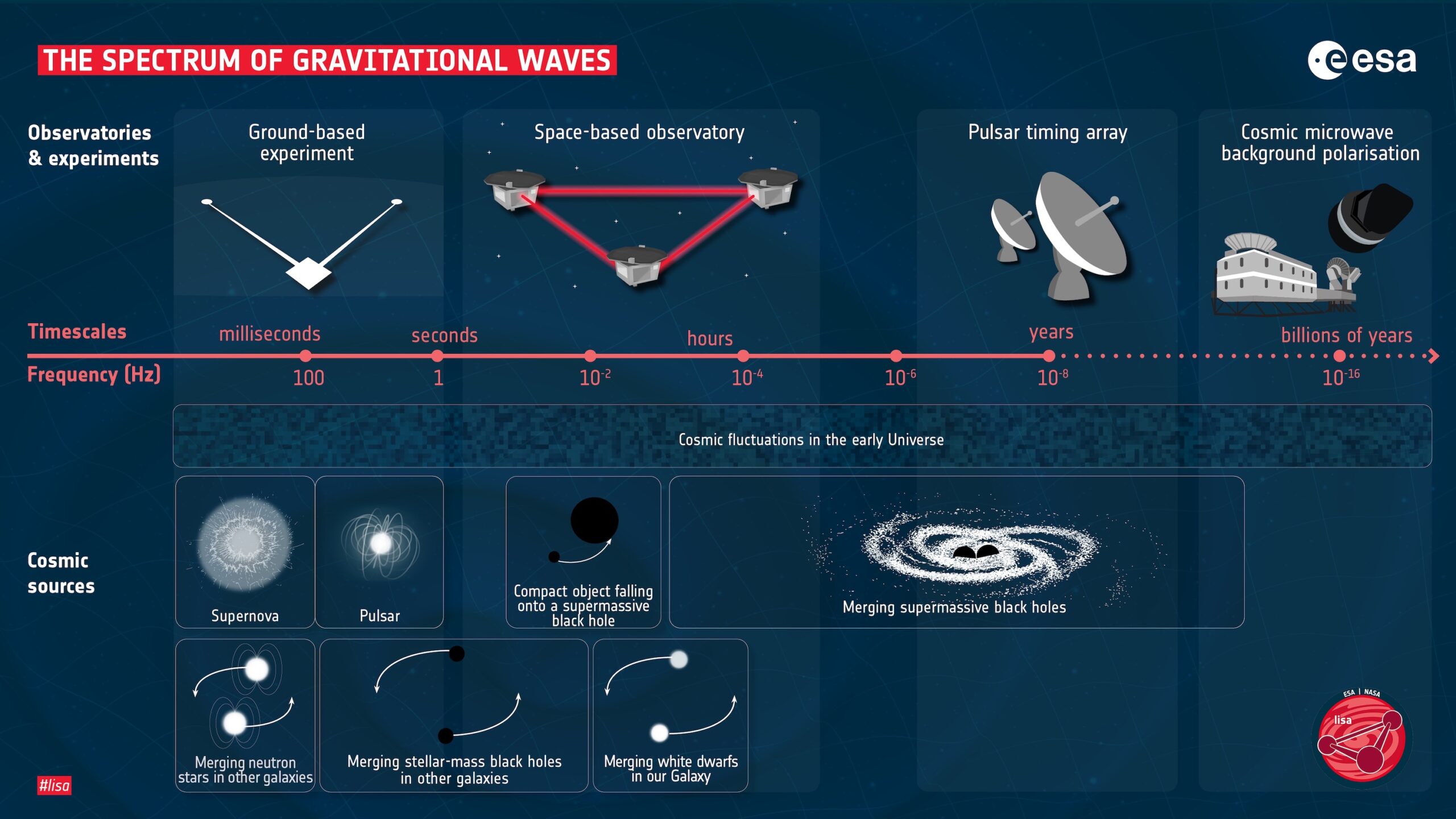
Infographic showing the typical frequency ranges of the gravitational waves produced by different sources. Click to enlarge. [ESA]
Simulating Gravitational Waves
Smadar Naoz (University of California, Los Angeles) and Zoltán Haiman (Columbia University) simulated the gravitational waves that would result from a stellar-mass black hole spiraling in to merge with one member of a supermassive black hole binary. This type of merger is called an extreme-mass-ratio inspiral. First, Naoz and Haiman estimated the number of extreme-mass-ratio inspirals as a function of the mass of the black holes in the binary system. Perhaps counterintuitively, stellar-mass black holes are much more likely to merge with the less massive black hole in a binary system, thanks to gravitational perturbations.
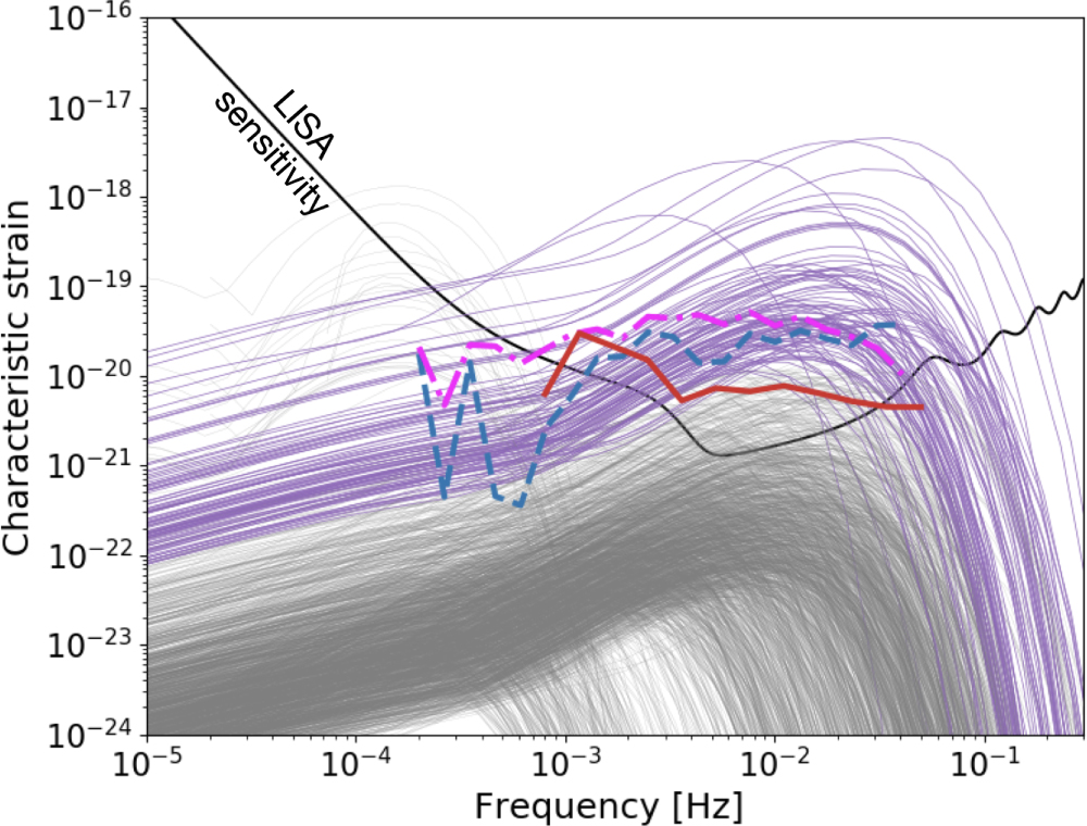
Predicted gravitational wave amplitude as a function of frequency for resolved (purple lines) and unresolved (grey lines) systems, compared to LISA’s estimated sensitivity. Click to enlarge. [Naoz & Haiman 2023]
Observing gravitational waves from a stellar-mass black hole as it spirals toward a supermassive black hole can help us understand many aspects of how supermassive black holes grow and merge. In particular, these observations may help us put a number on how many companions a supermassive black hole is likely to have; do these behemoths mostly fly solo, or are pairs, triples, or quartets more likely? Hopefully, it’s just a matter of time before LISA is in place in its berth in space — the planned launch date is 2037 — and ready to open a new window onto gravitational waves.
Citation
“The Enhanced Population of Extreme Mass-Ratio Inspirals in the LISA Band from Supermassive Black Hole Binaries,” Smadar Naoz and Zoltán Haiman 2023 ApJL 955 L27. doi:10.3847/2041-8213/acf8c9


