
New Spectral Signs of Buckyballs Discovered in Planetary Nebula
Fullerenes — a class of molecules composed entirely of interconnected carbon atoms — are the largest molecules definitively detected in space. Researchers using JWST to study a planetary nebula have found new spectral features from a fullerene composed of 60 carbon atoms, offering another way to study how these molecules form and survive in space.
Full of Fullerenes
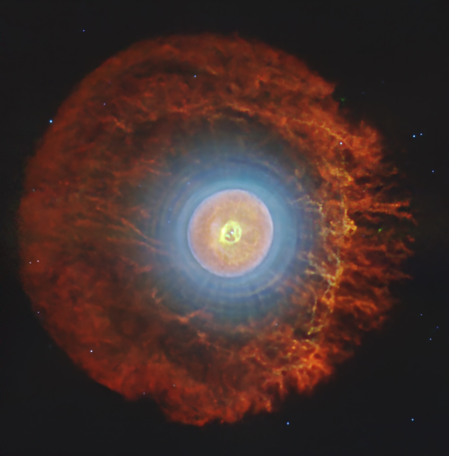
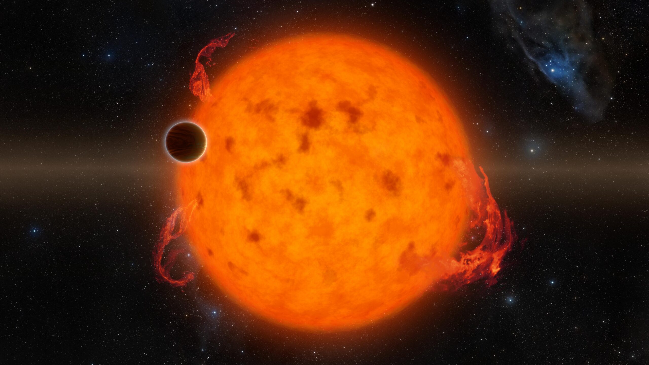
Planetary nebula Tc 1 as seen by JWST. [NASA / ESA / CSA / Western University, J. Cami]
Since that discovery, Tc 1 has been a hot spot for studies of buckyballs. However, researchers are still puzzling over how these large molecules form and survive in harsh space environments.
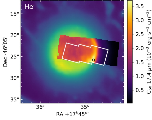
A closeup of the center of Tc 1, showing the region observed with JWST’s Mid-Infrared Instrument (black-to-yellow color scale) and Near-Infrared Spectrograph (white outline). The background color scale shows the nebula’s H-alpha emission as seen by the Very Large Telescope. [Adapted from Giese et al. 2026]
From Spitzer to JWST
Morgan Giese (The University of Western Ontario) and collaborators recently reported on the results of a JWST observing program that aimed to understand how fullerenes respond to changes in their environment. The team mapped the distribution of C60 molecules at varying distances from the powerful ionizing radiation of Tc 1’s central star.
The team successfully spotted the emission features from the fullerene C60 seen in earlier observations, but they also turned up something unexpected: a handful of prominent emission features from 3.5 to 5.2 microns that had not been reported previously.
Feature Presentation
What’s the source of these emission features? The distribution of the emission provides a strong clue: known spectral features from fullerenes C60 and C70 are concentrated in a narrow, bright ring around the center of the nebula, with diffuse emission suffusing the rest of the nebula — and the newfound spectral features follow the same distribution.
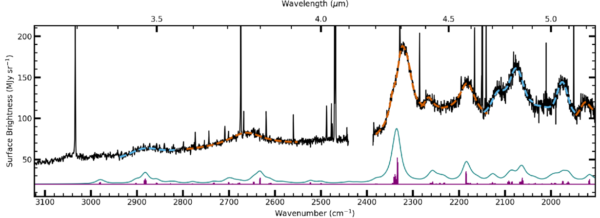
JWST spectrum of Tc 1 (black line) extracted from the area indicated by a black circle in the previous image. The orange and blue dashed lines show fits to the newfound emission bands, and the results of the anharmonic calculations are shown as the teal line below the JWST spectrum. Click to enlarge. [Giese et al. 2026]
Giese and coauthors found that 17% of the energy emitted by the C60 molecules in Tc 1 is released in these combination bands, suggesting that these features must be taken into account when modeling the cooling of C60 molecules. The discovery of new fullerene spectral features also has implications for future studies of these molecules: since these features appear in a wavelength range where features from other complex molecules like polycyclic aromatic hydrocarbons are weak, these newly identified bands provide a promising way to spot and study fullerenes across space environments.
Citation
“Detection of C60 Combination Bands in the Near-IR Spectrum of Tc 1,” Morgan M. Giese et al 2026 ApJL 1004 L32. doi:10.3847/2041-8213/ae76d5


.jpg)