The Sun’s activity history, the sources of tiny jets, and how magnetic fields might impact space weather forecasts: today’s Monthly Roundup introduces a trio of recent research articles from the Astrophysical Journal that tackle hot topics in solar physics.
From 1755 to 2020: Reconstructing Centuries of Solar Activity
Since the 1970s, regular monitoring of the Sun’s magnetic field has allowed researchers to decipher the Sun’s behavior as it cycles through periods of low and high activity. But what resources exist for studying the Sun’s past behavior? To investigate the long-term behavior of the Sun, researchers reach for historical records of sunspots, which stretch back to the 1700s.
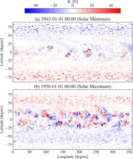
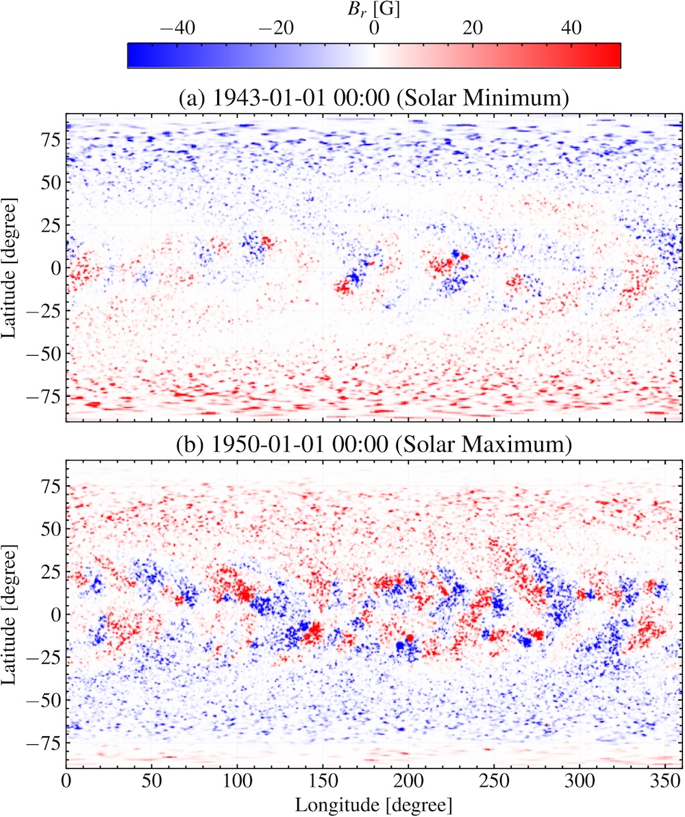
Example maps of the simulated photospheric radial magnetic field during a period of low (top) and high (bottom) solar activity. Click to enlarge. [Jha et al. 2026]
(Southwest Research Institute) and collaborators explored whether historical records and modern statistics could be used to reconstruct the behavior of the solar magnetic field centuries into the past. Jha’s team used recorded sunspot numbers from 1755 to 2020 as an input for their newly developed Synthetic Active Region Generator, which generates synthetic solar active regions based on known statistics of these regions. This catalog of active regions becomes the input for the Advective Flux Transport model, which simulates the active regions as they emerge and evolve, allowing for an estimation of the magnetic field across the Sun’s disk.
Jha and coauthors found that this method successfully reproduced the expected large-scale behavior of the Sun’s magnetic field across multiple solar cycles, such as the reversal of the polarity of the solar magnetic field near the peak of the activity cycle. While this work highlights the impressive results obtained from combining historical sunspot records with modern sunspot statistics, the team pointed out that this method cannot accurately reproduce all quantities because of the nonlinear nature of the underlying physics. Future work will refine the model further, and in the meantime, the team’s simulated historical magnetic field maps will be made publicly available.
Where Do the Tiniest Coronal Jets Come From?
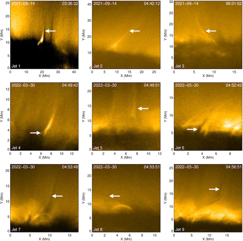
The Sun’s atmosphere is filled with an ever-shifting maze of magnetic field lines, which reconfigure and release pent-up magnetic energy in a process called magnetic reconnection. Magnetic reconnection can launch particles and heat plasma, and it’s thought to be responsible for driving jets on a variety of scales in the Sun’s tenuous outer atmosphere, or corona. Annu Bura (Indian Institute of Astrophysics; Pondicherry University) and coauthors investigated the physical origins of the smallest of these reconnection driven jets, picoflare jets, using data from the Extreme Ultraviolet Imager on board Solar Orbiter. Solar Orbiter has ventured within 0.3 au of the Sun, and its Extreme Ultraviolet Imager has returned exceptionally precise high-energy images of our home star.
Bura and collaborators identified picoflare jets by the presence of a hot, bright spire coupled with a cool, dark streak, forming a structure shaped like the letter “Y” upside down. They found that the bright and dark features were on average 650 and 490 kilometers wide, respectively, with a typical jet length of 16,900 kilometers. They also found that the bright features moved more quickly than the dark features, and the jets tended to last about 6 minutes. Overall, these measurements place the jets in between the scales expected for picoflare jets and slightly larger features called jetlets, though the energies are consistent with expectations for picoflare jets.
Using radiation magnetohydrodynamics simulations, the team explored the origins of their sample of jets. The simulations suggested that the bright features arose from hot, tenuous coronal plasma, while the accompanying dark features were due to cooler, denser plasma venturing upward from deeper in the Sun’s atmosphere, in the chromosphere. Overall, the simulations and observations support a picture in which picoflare-scale jets are driven by magnetic reconnection after magnetic flux emerges through the Sun’s surface. This echoes the formation route of larger coronal jets, suggesting that this process may apply to a wide range of physical scales.
Investigating the Influence of the Solar Polar Magnetic Field
The vast majority of our observations of the Sun have come from within a few degrees of the ecliptic plane, either from telescopes situated on Earth’s surface or from spacecraft that stuck close to the plane of our solar system. With rare but notable exceptions — the Ulysses spacecraft, which measured the Sun’s magnetic field and plasma environment from a near-polar orbit, and Solar Orbiter, which took the first-ever image of the Sun’s poles in November 2025 — the Sun’s poles have remained hidden from our instruments.
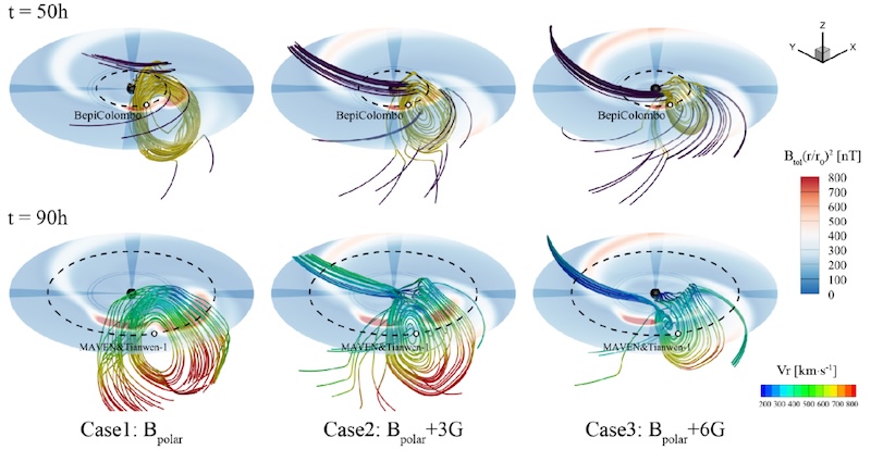
Our limited knowledge of the Sun’s polar magnetic field has consequences for our ability to model space weather events like coronal mass ejections. A team led by Xiao Zhang (Chinese Academy of Sciences; University of Chinese Academy of Sciences) has used numerical simulations to investigate how solar polar magnetic field conditions influence the propagation of a coronal mass ejection (CME) through the solar system.
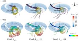
Simulation results showing how the propagation and expansion of a CME are affected by the polar magnetic field strength. Click to enlarge. [Zhang et al. 2026]
The team simulated a CME from 4 December 2021, which was observed by the BepiColombo spacecraft at Mercury and Tianwen-1 and MAVEN at Mars. The simulations showed that as the polar magnetic field strength increases, the CME’s movement through the solar system becomes slower. CMEs typically expand as they billow outward from the solar corona and sweep past the planets; increasing the polar magnetic field strength slowed the CME’s expansion as well. A stronger polar magnetic field also alters the background solar wind, making it slower and denser. Overall, these results demonstrate that the strength of the Sun’s poorly constrained polar magnetic field can have a significant impact on the movement and evolution of a CME. In future work, Zhang’s team plans to expand their investigation to a larger sample of CMEs.
Citation
“Historical Reconstruction of Solar Surface Magnetism from Cycles 1–24 Using the Synthetic Active Region Generator and the Advective Flux Transport Model,” Bibhuti Kumar Jha et al 2026 ApJ 997 279. doi:10.3847/1538-4357/ae279a
“On the Origin of Coronal Picoflare Jets,” Annu Bura et al 2026 ApJ 1000 94. doi:10.3847/1538-4357/ae48e6
“Influence of Solar Polar Magnetic Fields on the Propagation of Coronal Mass Ejections,” Xiao Zhang et al 2026 ApJ 1000 200. doi:10.3847/1538-4357/ae4c54