
Life Is Like a Box of Potential Biosignatures
Editor’s Note: Astrobites is a graduate-student-run organization that digests astrophysical literature for undergraduate students. As part of the partnership between the AAS and astrobites, we occasionally repost astrobites content here at AAS Nova. We hope you enjoy this post from astrobites; the original can be viewed at astrobites.org.
Title: The Detectability of CH4/CO2/CO and N2O Biosignatures Through Reflection Spectroscopy of Terrestrial Exoplanets
Authors: Armen Tokadjian, Renyu Hu, and Mario Damiano
First Author’s Institution: NASA’s Jet Propulsion Laboratory
Status: Published in AJ
Are we alone in the universe? This is one of the longest-standing questions ever asked by humankind. Though extraterrestrial life is discussed as a philosophical thought exercise, the NASA Astrophysics flagship mission of the 2040s, the Habitable Worlds Observatory (HWO), will get us closer than ever to the answer. This mission aims to detect signs of life on exoplanets. When active, the HWO will observe the atmospheres of Earth-like worlds to see if there are any particular molecules that could reveal past or present life. On Earth today, oxygen gas (O2) is a large component of our atmosphere and is considered a biosignature, since it is primarily produced as a byproduct of photosynthesis by living organisms. However, Earth’s atmosphere looked very different billions of years ago, when life had just begun to form. The authors of today’s article put forth theoretical models of how habitable exoplanets might appear to HWO using the molecules present in the Earth’s atmosphere from earlier eons, and test if HWO will be able to detect these molecules in simulated observations.
It’s Not Just a “Phase,” Mom, It’s an Eon
We all look different from the pictures from our youth, and Earth is no exception. And since life has been flourishing on Earth for billions of years, we can expect that any potentially life-harboring exoplanet may look like Earth from a different stage of its life. The authors of today’s article take two snapshots of Earth from two different phases, or eons, of its youth — but instead of revealing awkward braces and self-cut bangs, they are looking for the different molecules present in its early atmosphere. The first signs of life — microbes such as bacteria and archaea — emerged about 4 billion years ago during the Archean Eon. At this time, Earth’s atmospheric makeup was mostly nitrogen (N), carbon dioxide (CO2), and methane (CH4). Of these, CH4 is particularly interesting to astrobiologists because the primary source of CH4 during the Archean Eon was methanogenesis, a process that produces methane as a byproduct during microbial respiration, making CH4 a strong biosignature. However, abiotic processes like volcanism can produce CH4 as well. Therefore, the co-presence of CO has been suggested to distinguish the production mechanism of CH4, as volcanic activity typically produces more CO than CH4. A detection of CH4 in an atmosphere with a high CO to CH4 ratio should be considered a false positive of the CH4 biosignature as it is likely to have been produced abiotically.
In the following eon, the Proterozoic (2.5 billion to 541 million years ago), the atmospheric oxygen level began to rise, and the first eukaryotic organisms evolved. Microbes using the nitrogen cycle became the predominant producers of dinitrogen oxide (N2O), a compelling biosignature. Even more enticing is that N2O has few abiotic sources, unlike CH4. The authors of today’s article produced atmospheric models based on the biosignatures present in both the Archean and Proterozoic eons, and from those models tried to infer the presence of CH4/CO2/CO and N2O, respectively.
Earth as a Model
For both cases, the authors generated spectra using radiative transfer models, inputting parameters such as the cloud coverage, surface albedo (i.e., the fraction of light that a surface reflects), and the amount of the molecules of interest (specifically the number of a specific gas molecule divided by total number of molecules in a given volume). To model the Archean Earth atmosphere, the authors fix the amount of CH4 to be the upper limit of CH4 that could have been present in the Archean atmosphere, and they consider three different amounts of CO, corresponding to CO/CH4 ratios of 1, 5, and 10, respectively.
To model the Proterozoic Earth atmosphere, the authors consider two examples with different amounts of N2O. The first model corresponds to the upper limit of N2O for a Proterozoic Earth-like planet around a G-type star, and the second model corresponds to the same kind of planet, but around a K-type star instead. The K-type host star allows for much higher amounts of N2O in the planet’s atmosphere. This is because G-type stars are hotter and therefore have a higher ultraviolet flux, which causes the N2O in the atmosphere to photodissociate. These parameters are used in their radiative transfer model, which will produce a synthetic reflected light spectrum — i.e., the spectrum of light that is reflected off a cool exoplanet, which resembles what the HWO aims to observe.
Show Me the Biosignatures
To see if the authors can detect these molecules from these synthetic spectra, they employ an atmospheric retrieval code. In short, the synthetic reflection spectra generated by their radiative transfer model is sampled many, many times to see which one best fits the parameters of interest (most importantly, the presence of potential biosignatures). The planet-to-star flux ratio as a function of wavelength for the forward model with CO/CH4 = 10 along with the retrieval result for the Archean Earth atmosphere is shown in Figure 1. The authors find that they are able to detect CH4 and CO2 in the atmosphere, but they fail to constrain the CO abundance for any of the three cases. This is illustrated in Figure 1, where the CO features are relatively weak or located within a stronger CO2 feature. Because of this, it will be challenging to know if a potential detection is a false positive for the CH4/CO2 biosignature pair with similar observations.
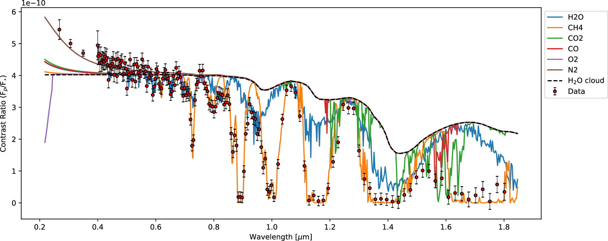
Figure 1: Planet-to-star flux ratio versus wavelength for Archean Earth-like planets with CO/CH4 = 10. The model is shown by the red circles and the retrieval result is overlaid. Each molecule of interest is labeled in a separate color to show the individual molecular contributions. While CH4 and CO2 are well constrained by the retrieval, CO is not. [Tokadjian et al. 2024]
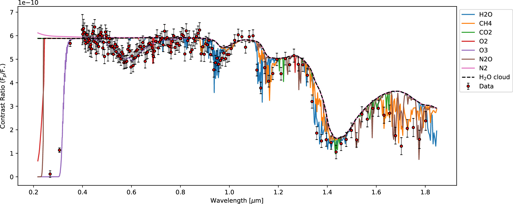
Figure 2: Same as Figure 1, but for the Proterozoic Earth-like planet around a K-type star. N2O is well constrained by the retrieval result. [Tokadjian et al. 2024]
Original astrobite edited by Kylee Carden.
About the author, Tori Bonidie:
I am a 4th-year PhD candidate studying exoplanets at the University of Pittsburgh. Prior to this, I earned my BA in astrophysics at Franklin and Marshall College, where I worked on pulsar detection as a member of NANOGrav. In my free time you can find me cooking, napping with my cat, or reading STEMinist romcoms!


")


