Making It Rain in the Circumgalactic Medium
Editor’s note: Astrobites is a graduate-student-run organization that digests astrophysical literature for undergraduate students. As part of the partnership between the AAS and astrobites, we occasionally repost astrobites content here at AAS Nova. We hope you enjoy this post from astrobites; the original can be viewed at astrobites.org.
Title: The Impact of Enhanced Halo Resolution on the Simulated Circumgalactic Medium
Authors: Cameron B. Hummels, Britton D. Smith, Philip F. Hopkins, et al.
First Author’s Institution: TAPIR, California Institute of Technology
Status: Submitted to ApJ
It can be easy to think of galaxies as islands in the universe, floating around in isolation. However, a galaxy is actually surrounded by a huge sea of low-density gas that extends out to its virial radius and beyond. This gas is known as the circumgalactic medium (CGM), and more and more research is showing that the CGM has a crucial role to play in galaxy evolution. Observing the CGM has proven difficult due to its extremely low density, though, so simulations have played a large role in understanding the physics of this region. In today’s paper, the authors detail the effects of running a CGM simulation with significantly increased resolution, capable of resolving cool gas that precipitates in the CGM and rains down on the galaxy.
What Do We Know About the CGM?
Residing just outside of the galaxy, the CGM is home to large-scale flows of gas that drive galaxy evolution. These gas flows provide fuel for star formation, regulate the interactions between dark matter halos and the intergalactic medium, and contain the energy, mass, and metals of large outflows from a galaxy. In fact, the CGM is predicted to hold at least as many baryons and heavy elements as galaxies themselves, and most of the metals in the universe are found in the CGM. These metals (meaning anything heavier than hydrogen or helium in astronomy terms), deposited by galactic outflows, serve as the dominant coolant for the CGM. They are capable of radiating energy away more easily than elements like hydrogen, so an increased abundance of metals can lead to cooler gas. Consequently, this influx of metals helps to create two phases of gas: “cool” (10,000 Kelvin) gas composed of neutral hydrogen and other elements in low-energy ionization states, and “hot” (300,000–1,000,000 Kelvin) gas that contains oxygen, nitrogen, and neon in high-energy ionization states.
Unfortunately, computational work has chronically underproduced the observed abundances of these ions across redshifts by orders of magnitude. Recent work has shown that AGN feedback can increase the abundances of oxygen and other ions in the hot gas, but the discrepancy remains for hydrogen and other ions in the cool gas. In today’s paper, the authors discuss the effect of increased simulation resolution on these discrepancies.
Resolving the Resolution Issue
Perhaps one reason that simulations struggle to reproduce observations of the CGM lies in their resolution limits. Similar to how using more pixels in a television or computer screen gives a better image, increasing the resolution in a simulation means using more cells or particles to obtain a better physical picture of what is going on. However, each increase in resolution increases the computational cost of the simulation. This means your simulation that took a few days to run could instead take a few months.
Consequently, most simulations of galaxies apply their highest resolution to regions of high density where most of the matter is. This is great for figuring out what happens in the dense disk of a galaxy, but not ideal for studying the low-density CGM. Today’s paper runs simulations that force high resolution upon the CGM, reaching resolutions that are comparable to those normally obtained in the disk of the galaxy. This technique is appropriately named Enhanced Halo Resolution (EHR). Figure 1 shows the resolutions obtained by both a normal cosmological simulation and an EHR one for a region encompassing a galaxy and its surrounding filaments.
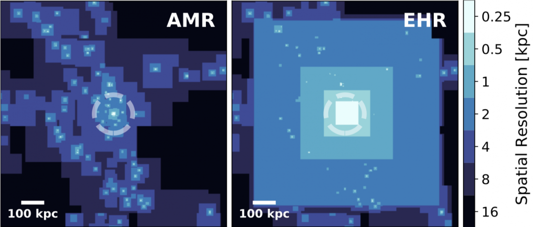
Figure 1: Plots of resolution for a traditional (AMR — adaptive mesh refinement) and EHR simulation. Each of these grids is made up of many cells, and spatial resolution refers to the physical length (in kiloparsecs) of the smallest cell that is present in a region. In the left panel, many galaxies are present and a particularly massive galaxy lies at the center. Its virial radius is shown by the dotted white line. Resolution in the CGM is roughly 16 times worse than in the disk of the galaxy. On the right, the EHR simulation enforces high resolution approximately to the virial radius, ensuring that interactions within the CGM are given much more computational attention. [Hummels et al. 2019]
What Does this Computational Cost Buy You?
By better resolving the gas in the CGM, the authors note that a number of physical effects present themselves. Firstly, the balance of cool and hot gas is shifted, leaving more cool gas and less hot gas than in simulations with lower resolution. The clouds of cool gas that form are also greater in number and smaller in size. Finally, the amount of neutral hydrogen and other low-energy ions found in the cool gas increases, while the abundances of oxygen, nitrogen, and neon in high-energy ionization states fall due to the decrease in hot gas. Coupled with the aforementioned work on AGN feedback, this can bring simulations closer to the observed abundances for these ions.
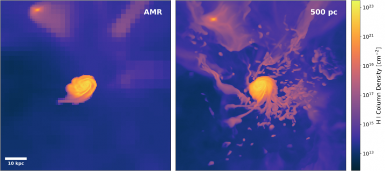
Figure 2: A galaxy and the CGM in an AMR simulation and an EHR one. A significant increase in HI (neutral hydrogen) can be seen in the EHR simulation. Recall that neutral hydrogen tracks the cool gas, which condenses into many clumps on the right that weren’t resolved in a traditional AMR simulation. Many of these clumps fall back into the galaxy because they no longer have enough thermal energy to resist the gravitational pull of the galaxy. [Hummels et al. 2019]
Why does an increase in resolution result in more cool gas? The answer lies in how gas mixes in simulations. With lower resolution, clouds of cool gas are typically resolved only by a few cells, inducing artificial mixing between the hot and cool gas. The authors perform a test simulation demonstrating this, shown in Figure 3.
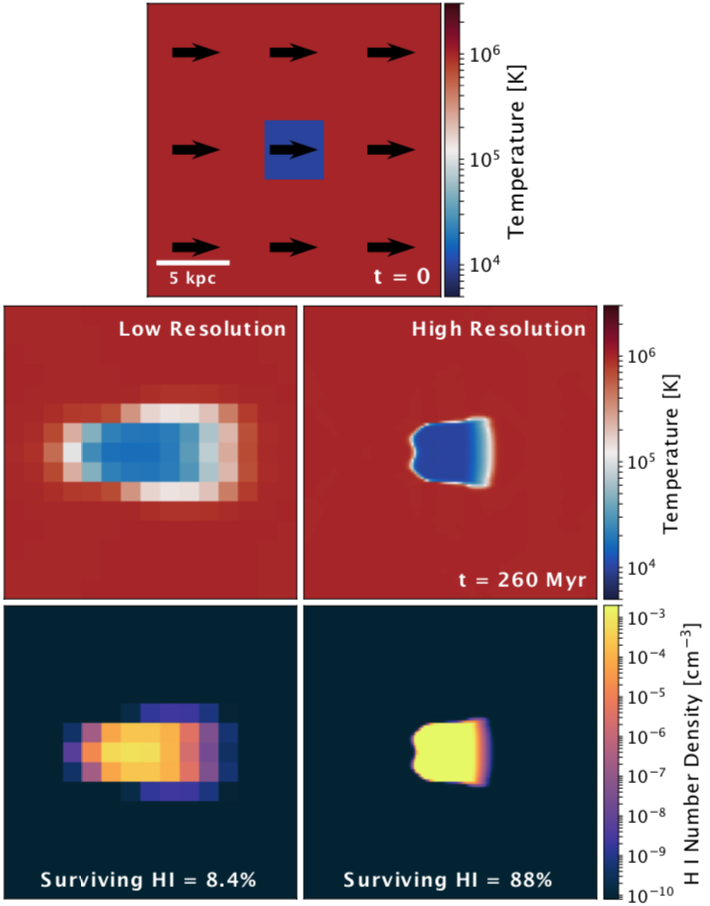
Figure 3: In this test problem, a 4-kiloparsec-wide cloud of cool gas sits in a flow of hot gas for 260 million years. In the low-resolution test, the boundary of the cloud is only resolved by a few cells. This artificially thick boundary means that much of the cool gas quickly mixes with the hot gas and eliminates the HI (neutral hydrogen). In the high-resolution case, the boundary becomes much thinner, allowing the interior cool gas to survive much longer. [Hummels et al. 2019]
About the author, Michael Foley:
I’m a graduate student studying Astrophysics at Harvard University. My research focuses on using simulations and observations to study stellar feedback — the effects of the light and matter ejected by stars into their surroundings. I’m interested in learning how these effects can influence further star and galaxy formation and evolution. Outside of research, I’m really passionate about education, music, and free food.