Tuning In to Reveal Stellar Wobbles
Editor’s note: Astrobites is a graduate-student-run organization that digests astrophysical literature for undergraduate students. As part of the partnership between the AAS and astrobites, we occasionally repost astrobites content here at AAS Nova. We hope you enjoy this post from astrobites; the original can be viewed at astrobites.org.
Title: An astrometric planetary companion candidate to the M9 Dwarf TVLM 513−46546
Authors: Salvador Curiel et al.
First Author’s Institution: National Autonomous University of Mexico (UNAM)
Status: Published in AJ
Finding Planets
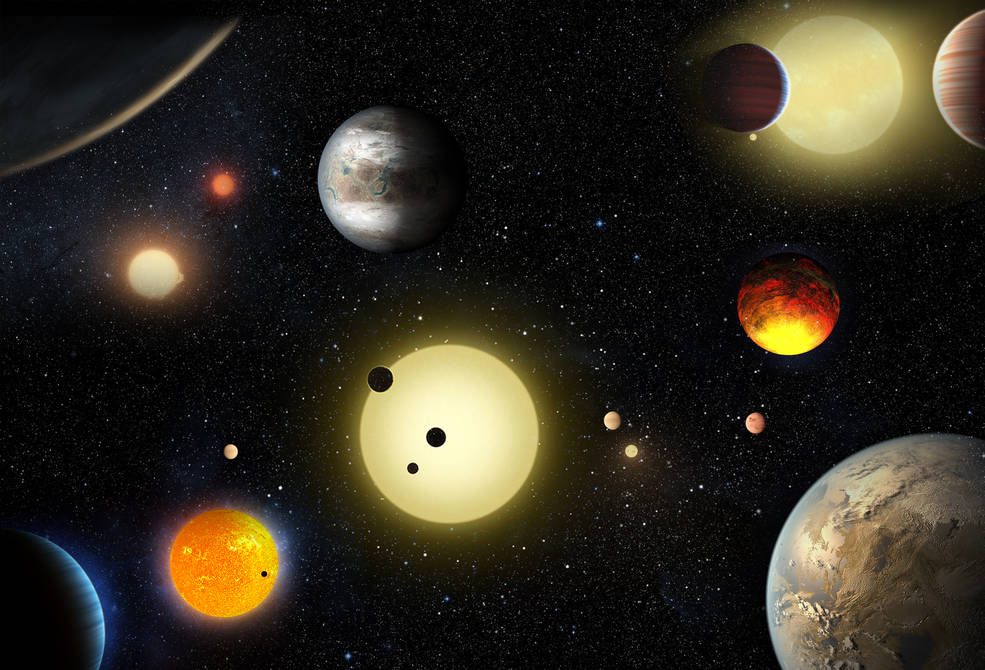
This artist’s illustration depicts multiple examples of planetary systems we’ve discovered. [NASA/W. Stenzel]
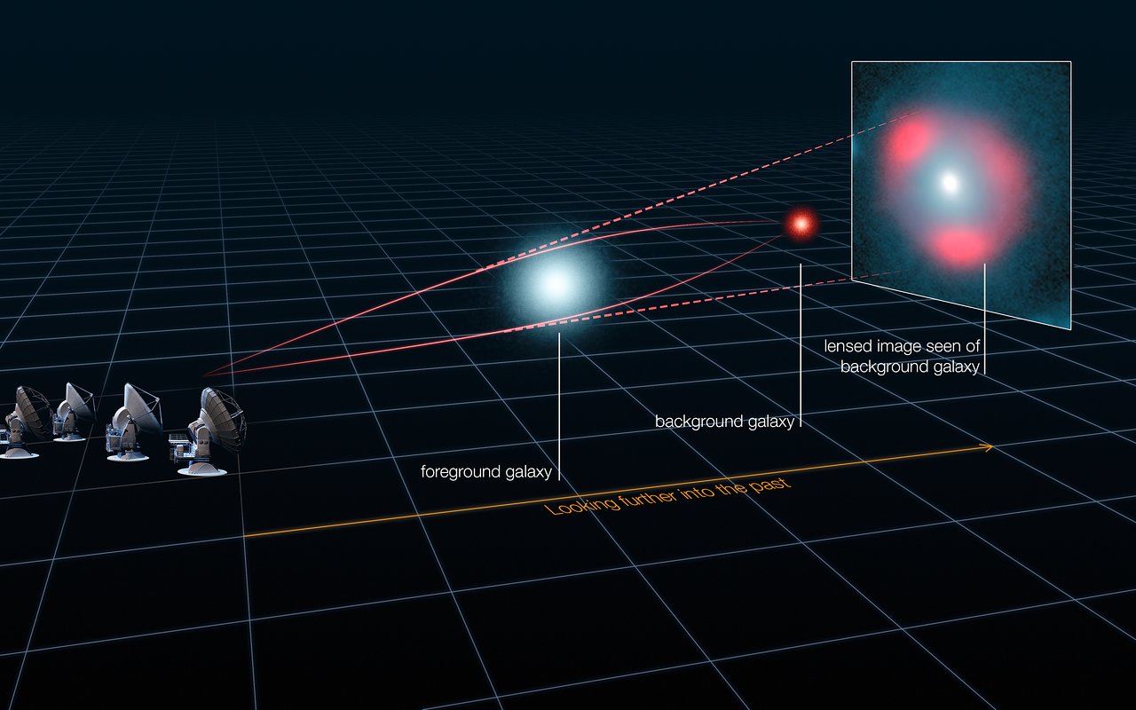
However, these are not the only methods we can use to find planets. Astronomers have also made use of the light-bending power of gravity (known as microlensing) to find planets, which is a major science goal of the upcoming Nancy Grace Roman Space Telescope. Sometimes, it is even possible to directly image a planet if the light of the host star can be blocked. Combined, these various methods have allowed us to find more than 4,000 exoplanets orbiting stars other than our Sun.
Wobbly Stars
There is one exoplanet detection method that we haven’t discussed yet, known as the astrometric method. This method essentially looks at the position of a star over a period of time and tracks deviations from the expected position. Discovering a planet this way requires excellent precision though. Fortunately, the Gaia satellite is capable of making such a measurement, and it is expected that by the end of the mission that we will find many new planets through this method (for more details see this bite). With that said, there is only one currently claimed discovery of an exoplanet through astrometry. Today’s paper increases that count to two!
M dwarfs, stars cooler than our Sun, are one of the major targets for exoplanet searches due to their large numbers in our galaxy and the fact that habitable exoplanets around M-dwarfs are some of the best candidates for atmospheric characterization. In this paper, the authors look at the M9 dwarf TVLM 513 (with a mass of 0.06–0.08 solar mass), which had been a target for earlier studies in the radio using very-long-baseline interferometry (VLBI). The authors combine archival VLBI data with new observations to produce the stellar motions shown in Figure 1.
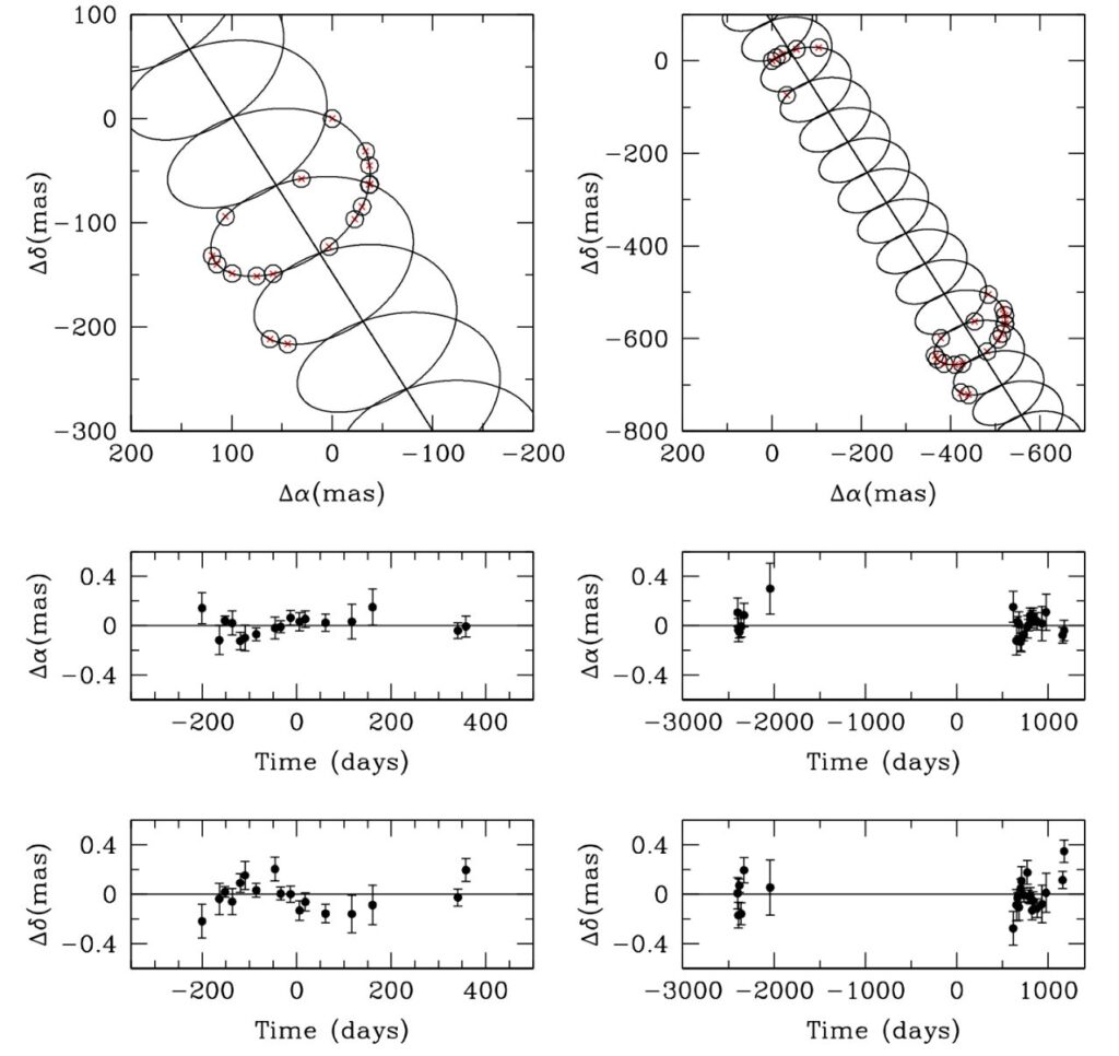
Figure 1: Parallax fits to the VLBI data. The left panels are the new data and the right panels are the combined archival+new data. The upper panels show the fit using only the proper motions and the parallax of TVLM 513. The middle panels show the residuals in right ascension and the bottom panels show the residuals in declination. The temporal trend in the residuals suggests the presence of a companion. [Curiel et al. 2020]
In Figure 1, there are two clear types of motion of TVLM 513. The first is the general motion from the upper left to the bottom right, caused by the proper motion of the star on the sky. The second is a back-and-forth motion known as parallax, which is caused by the Earth’s orbit around the Sun. At first glance, the observed positions of the star appear to follow these two general trends well, but there are small deviations from this path that are shown in the bottom two panels of Figure 1. This tells the authors that there is something tugging on their star, which in this case turns out to be a planet!
From their fits to the observed astrometric signal, the authors find a companion at a period of P = 221 ± 5 days, with a circular orbit, a mass of m = 0.35−0.42 Jupiter masses, a semi-major axis of a = 0.28−0.31 au, and an inclination angle of i = 71−88° (where 0° is face-on and 90° is edge-on). This discovery of the planet TVLM 513b is only the second astrometric discovery of a planet to date. It is also the first planet detection to use radio astrometry.
TVLM 513b in Context
With a new (Saturn-like) planet in hand, the authors turn towards the wealth of exoplanet observations to understand how their exciting new discovery fits in with the broader picture. To do this, the authors create Figure 2, which compares the host stellar mass to the planetary mass and the semi-major axis of the planet’s orbit. In comparison to most known planets, TVLM 513b orbits a much lower-mass star. While the TESS mission will begin to add new planets discovered around other low-mass stars, astrometry will continue to be an effective method for finding planets around such stars. TVLM 513b itself is somewhat moderate in terms of its mass and semi-major axis compared to other planets. Combined, this system lies in a relatively unexplored region of parameter space. Most other planets in this region were found using microlensing, which unfortunately does not allow for detailed follow-up observations.
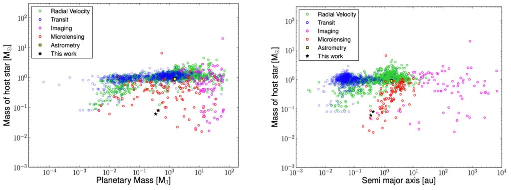
Figure 2: Comparison of fundamental properties of planets and their orbits as a function of discovery method. Left: Comparison of stellar mass and planetary mass. Right: Comparison of stellar mass and semi-major axis of the planet. In both panels, green points are radial velocity, blue are transit, pink are imaging, red are microlensing, and yellow are astrometry discoveries. The black stars are the location of TVLM 513b using the upper and lower mass limits for the host star. [Curiel et al. 2020]
The authors also note that the parameters of this planet are somewhat unexpected given commonly accepted theories of planet formation. The two main theories for the creation of giant planets are core accretion and disk instability. For core accretion, the masses of planets should scale with their host star, so a massive planet around such a low mass star is unexpected. While disk instability can create massive planets around low mass stars, both models predict massive planets to occur at least a few au from the central star, whereas TVLM 513b has a semi-major axis of ~0.3 au. The authors note that planet could have formed farther out and migrated in — but how and why did it stop at 0.3 au?
In brief, the authors of today’s paper have found a new planet through radio astrometry. But their discovery amounts to more than that. It is further proof that astrometry can not only find planets, but prompt new questions that will continue to drive the exoplanet field forward. This planet, combined with the many that continued TESS and Gaia observations and future missions will yield, will answer outstanding questions and pose even harder ones as we try to understand the origins of planetary systems both far away and closer to home.
About the author, Jason Hinkle:
I am a graduate student at the University of Hawaii, Institute for Astronomy. My current research is on multi-wavelength photometric and spectroscopic follow-up of tidal disruption events. My research interests also include a number of topics related to AGN, including outflows, X-ray spectroscopy, and multi-wavelength variability. In addition to my love for astronomy, I enjoy hiking, sports, and musicals.


 Stars")